
Efficient Algorithms for Simplicial Complexes Used in the Computation
of Lyapunov Functions for Nonlinear Systems
Sigurdur Freyr Hafstein
Faculty of Physical Sciences, University of Iceland, Dunhagi 5, 107 Reykjavik, Iceland
Keywords:
Simplicial Complex, Triangulation, Algorithm, Lyapunov Function, Nonlinear System, Discrete-time System.
Abstract:
Several algorithms have been suggested to parameterize continuous and piecewise affine Lyapunov functions
for nonlinear systems in various settings. In these algorithms linear constraints are formulated for the val-
ues of a Lyapunov function at all vertices of a simplicial complex. They are then either solved using convex
optimization or computed by other means and then verified. Originally these algorithms were designed for
continuous-time systems and their adaptation to discrete-time systems and control systems poses some chal-
lenges in designing and implementing efficient algorithms and data structures for simplicial complexes. In this
paper we discuss several of these and give efficient implementations in C++.
1 INTRODUCTION
A Lyapunov function V for a dynamical system is a
continuous function from the state-space to the real
numbers that is decreasing along the system’s trajec-
tories. For a continuous-time system given by a dif-
ferential equation x
0
= f(x) this can be ensured by the
condition ∇V (x)
•
f(x) < 0. For a discrete-time system
x
k+1
= g(x
k
) a corresponding condition is
∆
g
V (x) := V (g(x)) −V (x) < 0.
In (Giesl and Hafstein, 2014a; Hafstein et al.,
2014; Li et al., 2015) novel algorithms for the compu-
tation of Lyapunov functions for nonlinear discrete-
time systems were presented. In these algorithms the
relevant part of the state-space is first triangulated,
i.e. subdivided into simplices, and then a continu-
ous and piecewise affine (CPA) Lyapunov function is
parameterized by fixing its values at the vertices of
the simplices. These algorithms resemble earlier al-
gorithms for the computation of Lyapunov functions
for nonlinear continuous-time systems, cf. e.g. (Ju-
lian, 1999; Julian et al., 1999; Marin
´
osson, 2002a;
Marin
´
osson, 2002b; Hafstein, 2007; Giesl and Haf-
stein, 2014c; Bj
¨
ornsson et al., 2014), referred to as
the CPA algorithm. The essential idea is to formulate
the conditions for a Lyapunov function as linear con-
straints in the values of the Lyapunov function to be
computed at the vertices of the simplices of the sim-
plicial complex.
The implementation of these algorithms for
discrete-time systems and continuous-time systems
can largely be done in similar ways. One first con-
structs a simplicial complex that triangulates the rel-
evant part of the state-space. Then an appropriate
linear programming problem for the system at hand
is constructed, of which every feasible solution pa-
rameterizes a Lyapunov for the system. Then one
either uses a linear programming solver, e.g. GLPK
or Gurobi, to search for a feasible solution, or one
uses a different method to compute values that can be
expected to fulfill the constraints and then verifies if
these values constitute a feasible solution to the linear
programming problem.
The non-locality of the dynamics in the discrete-
time case, however, poses an additional challenge
in implementing the algorithms in an efficient way.
Namely, whereas ∇V (x)
•
f(x) < 0 for a continuous-
time system is a local condition that can be formulated
as linear constraints for each simplex, the condition
V (g(x)) −V (x) < 0 for a discrete-time system is not
local. For a vertex x of a simplex S
ν
in the triangula-
tion T we must be able find a simplex S
µ
∈ T such
that g(x) ∈ S
µ
to formulate this condition as a linear
constraint. For triangulations consisting of many sim-
plices a linear search is very inefficient and therefore
more advanced methods are called for. The first con-
tribution of this paper is an algorithm that efficiently
solves this problem for fairly general simplicial com-
plexes appropriate for our problem of computing Lya-
punov functions.
The CPA algorithm has additionally been adapted
398
Hafstein, S.
Efficient Algorithms for Simplicial Complexes Used in the Computation of Lyapunov Functions for Nonlinear Systems.
DOI: 10.5220/0006480003980409
In Proceedings of the 7th International Conference on Simulation and Modeling Methodologies, Technologies and Applications (SIMULTECH 2017), pages 398-409
ISBN: 978-989-758-265-3
Copyright © 2017 by SCITEPRESS – Science and Technology Publications, Lda. All rights reserved

to compute Lyapunov functions for differential inclu-
sions (Baier et al., 2012) and control Lyapunov func-
tions (Baier and Hafstein, 2014) in the sense of the
Clarke subdifferential (Clarke, 1990). The next log-
ical step is to compute control Lyapunov functions
in the sense of the Dini subdifferential, a work in
progress with very promising first results. For these
computations one needs information on the common
faces of neighbouring simplices in the simplicial com-
plex and, in case of the Dini subdifferential, detailed
information on normals of the hyperplanes separating
neighbouring simplices. Efficient algorithms and data
structures for these computations are presented. This
is the second contribution of this paper.
The third contribution are algorithms to compute
circumscribing hyperspheres of the simplices of the
simplicial complex. These can be used to imple-
ment more advanced algorithms for the computation
of Lyapunov functions for discrete-time systems, a
work in progress.
Before we describe our algorithms in Section 2.1
and Section 3, we first discuss suitable triangulations
for the computation of CPA Lyapunov functions in
Section 2. In Section 3.2 we additionally analyse the
efficiency of our algorithm to search fast for simplices
and in Section 4 we give a few concluding remarks.
1.1 Notation
We denote by Z, N
0
, R, and R
+
the sets of the inte-
gers, the nonnegative integers, the real numbers, and
the nonnegative real numbers respectively. We write
vectors in boldface, e.g. x ∈R
n
and y ∈ Z
n
, and their
components as x
1
,x
2
,.. ., x
n
and y
1
,y
2
,.. ., y
n
. All
vectors are assumed to be column vectors. An in-
equality for vectors is understood to be component-
wise, e.g. x < y means that all the inequalities x
1
<
y
2
, x
2
< y
2
,.. ., x
n
< y
n
are fulfilled. The null vector in
R
n
is written as 0 and the standard orthonormal basis
as e
1
,e
2
,.. ., e
n
, i.e. the i-th component of e
j
is equal
to δ
i, j
, where δ
i, j
is the Kronecher delta, equal to 1 if
i = j and 0 otherwise. The scalar product of vectors
x,y ∈R
n
is denoted by x
•
y, the Euclidian norm of x is
denoted by kxk
2
:=
√
x
•
x, and the maximum norm of
x is denoted by kxk
∞
:= max
i=1,2,...,n
|x
i
|. The trans-
pose of x is denoted by x
T
and similarly the transpose
of a matrix A ∈ R
n×m
is denoted by A
T
. If A ∈ R
n×n
is an invertible matrix we denote its inverse by A
−1
and the inverse of its transpose by A
−T
. In the rest of
the paper n and in the code the global variable const
int n is the dimension of the Euclidian space we are
working in.
We write sets K ⊂ R
n
in calligraphic and we de-
note the closure, interior, and the boundary of K by
K , K
◦
, and ∂K respectively.
The convex hull of an (m + 1)-tuple
(v
0
,v
1
,.. ., v
m
) of vectors v
0
,v
1
,.. ., v
m
∈ R
n
is
defined by
co(v
0
,v
1
,.. ., v
m
) :=
(
m
∑
i=0
λ
i
v
i
: 0 ≤ λ
i
,
m
∑
i=0
λ
i
= 1
)
.
If v
0
,v
1
,.. ., v
m
∈R
n
are affinely independent, i.e. the
vectors v
1
−v
0
,v
2
−v
0
,.. ., v
m
−v
0
are linearly in-
dependent, the set co(v
0
,v
1
,.. ., v
m
) is called an m-
simplex. For a subset {v
i
0
,v
i
1
,.. ., v
i
k
}, 0 ≤ k < m,
of affinely independent vectors {v
0
,v
1
,.. ., v
m
}, the
k-simplex co(v
i
0
,v
i
1
,.. ., v
i
k
) is called a k-face of the
simplex co(v
0
,v
1
,.. ., v
m
). Note that simplices are
usually defined as convex combinations of vectors in
a set and not of ordered tuples, i.e. co{v
0
,v
1
,.. ., v
m
}
rather than co(v
0
,v
1
,.. ., v
m
). For the implementation
of the simplicial complexes below it is however very
useful to stick to ordered tuples.
In the algorithms we make heavy use of the
Standard C++ Library and the Armadillo lin-
ear algebra library (Sanderson, 2010). Very
good documentation on Armadillo is available at
http://arma.sourceforge.net and some comments on
its use for the implementation of the basic simpli-
cial complex in Section 2 are also given in (Hafstein,
2013). The vector and matrix types of Armadillo we
use in this paper are ivec, vec, and mat, which rep-
resent a column vector of int, a column vector of
double, and a matrix of double respectively.
2 SIMPLICIAL COMPLEX T
std
N,K
The basic simplicial complex T
std
N,K
and its efficient
implementation is described in (Hafstein, 2013). For
completeness we recall its definition but refer to (Haf-
stein, 2013) for the details.
To define the simplicial complex T
std
N,K
we first
need a few definitions.
An admissible triangulation of a set C ⊂R
n
is the
subdivision of C into n-simplices, such that the inter-
section of any two different simplices in the subdivi-
sion is either empty or a common k-face, 0 ≤ k < n.
Such a structure is often referred to as a simplicial n-
complex.
For the definition of T
std
N,K
we use the set S
n
of
all permutations of the numbers 1,2, .. .,n, the char-
acteristic functions χ
J
(i) equal to one if i ∈ J and
equal to zero if i /∈ J . Further, we use the functions
R
J
: R
n
→ R
n
, defined for every J ⊂ {1,2, ... ,n} by
R
J
(x) :=
n
∑
i=1
(−1)
χ
J
(i)
x
i
e
i
.
Efficient Algorithms for Simplicial Complexes Used in the Computation of Lyapunov Functions for Nonlinear Systems
399

Thus R
J
(x) puts a minus in front of the i-th coordinate
of x whenever i ∈ J .
To construct the triangulation T
std
N,K
, we first define
the triangulations T
std
N
and T
std
K,fan
as intermediate
steps.
Definition of T
std
N,K
1. For every z ∈ N
n
0
, every J ⊂ {1,2,. .. ,n}, and ev-
ery σ ∈ S
n
define the simplex
S
zJ σ
:= co(x
zJ σ
0
,x
zJ σ
1
,.. ., x
zJ σ
n
) (1)
where
x
zJ σ
i
:= R
J
z +
i
∑
j=1
e
σ( j)
!
(2)
for i = 0,1,2, ... ,n,.
2. Let N
m
,N
p
∈ Z
n
, N
m
< 0 < N
p
, and define the
hypercube N := {x ∈ R
n
: N
m
≤ x ≤ N
p
}. The
simplicial complex T
std
N
is defined by
T
std
N
:= {S
zJ σ
: S
zJ σ
⊂ N }. (3)
3. Let K
m
,K
p
∈ Z
n
, N
m
≤ K
m
< 0 < K
p
≤ N
p
, and
consider the intersections of the n-simplices S
zJ σ
in T
std
N
and the boundary of the hypercube K :=
{x ∈R
n
: K
m
≤ x ≤K
p
}. We are only interested
in those intersections that are (n −1)-simplices,
i.e. co(v
1
,v
2
,.. ., v
n
) with exactly n-vertices. For
every such intersection add the origin as a vertex
to it, i.e. consider co(0,v
1
,v
2
,.. ., v
n
). The set of
such constructed n-simplices is denoted T
std
K,fan
. It
is a triangulation of the hypercube K .
4. Finally, we define our main simplicial complex
T
std
N,K
by letting it contain all simplices S
zJ σ
in
T
std
N
, that have an empty intersection with the in-
terior K
◦
of K , and all simplices in the simplicial
fan T
std
K,fan
. It is thus a triangulation of N having a
simplicial fan in K .
The term simplicial fan of the triangulation of the hy-
percube K := {x ∈ R
n
: K
m
≤ x ≤ K
p
} seems nat-
ural, for mathematically it is a straightforward exten-
sion of the 3D graphics primitive triangular fan to ar-
bitrary dimensions. For a graphical presentation of
the complex T
std
N,K
with n = 2 see Figure 1. For fig-
ures of the complex with n = 3 see Figures 2 and 3 in
(Hafstein, 2013).
The class that implements the the basic simplicial
complex T
std
N,K
is T std NK. It is defined as follows:
struct T_std_NK {
ivec Nm,Np,Km,Kp;
Grid G;
int Nr0;
vector<ivec> Ver;
vector<vector<int>> Sim;
Figure 1: The simplicial complex T
std
N,K
in two dimensions
with K
m
= (−4, −4)
T
,K
p
= (4, 4)
T
,N
m
= (−6, −6)
T
, and
N
p
= (6,6)
T
.
vector<zJs> NrInSim;
vector<int> Fan;
int InSimpNr(vec x); // -1 if not found
bool InSimp(vec x,int s);
T_std_NK(ivec Nm,ivec Np,ivec Km,ivec Kp);
// added since (Hafstein, 2013) below
vector<list<int>> SimN;
vector<list<int>> SCV;
vector<list<vector<int>>> Faces;
vector<int> BSim;
int SVerNr(int s,int i);
ivec SVer(int s,int i);
};
Nm= N
m
and Np= N
p
define the hypercube N and
Km= K
m
and Kp= K
p
define the hypercube K .
vector<ivec> Ver is a vector containing all the
vertices of all the simplices in the complex, int
Nr0 is such that Ver[Nr0] is the zero vector, and
vector<vector<int>> Sim is a vector containing
all the simplices of the complex. A simplex is
basically an ordered tuple of (n + 1) vertices. Each
simplex is stored as a vector of (n + 1)-integers,
the integers refereing to the positions of the cor-
responding vertices in vector<ivec> Ver. G is a
grid defined by ivec Nm and ivec Np that is used
to enumerate all relevant vertices for T std NK and
vector<zJs> NrInSim and vector<int> Fan are
auxiliary structures that allow for the fast computa-
tion of a simplex S
ν
=Sim[s] such that x ∈S
ν
for an
arbitrary vector x ∈ R
n
. Their properties and imple-
mentation is described in detail in (Hafstein, 2013).
vector<list<int>> SimN, vector<list<int>>
SCV, vector<list<vector<int>>> Faces, and
vector<int> BSimp are new variables in the
class T std NK. Their purpose and initialization is
described in the next section.
SIMULTECH 2017 - 7th International Conference on Simulation and Modeling Methodologies, Technologies and Applications
400

2.1 Added Functionality in T std NK
In this section we describe the functionality that has
been added to the class T std NK since (Hafstein,
2013). From now on we denote the basic simpli-
cial complex T
std
N,K
by T . Further we denote the set
of all its vertices by V
T
and its domain by D
T
:=
S
S
ν
∈T
S
ν
.
Originally we fell back on linear search if x ∈ R
n
was in the simplicial fan of T
std
N,K
. Under the premise
that the simplicial fan is much smaller than the rest
of the simplicial complex this is a reasonable strat-
egy. Therefore we did not add a fast search structure
zJs to vector<zJs> NrInSim for simplices in the
fan. However, for a simplicial complex for which this
premise is not fulfilled, an improved strategy short-
ens the search time considerably. This might also
be of importance to different computational meth-
ods for Lyapunov functions that use conic partitions
of the state-space, a topic that has obtained consid-
erable attention cf. e.g. (Polanski, 1997; Branicky,
1998; Johansson and Rantzer, 1998; Johansson, 1999;
Polanski, 2000; Ohta, 2001; Ohta and Tsuji, 2003;
Yfoulis and Shorten, 2004; Lazar, 2010; Lazar and
Joki
´
c, 2010; Lazar and Doban, 2011; Ambrosino and
Garone, 2012; Lazar et al., 2013).
We achieve this by first adding such simplices
to the vector<zJs> NrInSim vector with appro-
priate values for z, J , and σ. This is very sim-
ple to make: In CODE BLOCK 1 in (Hafstein, 2013)
directly after Fan.push back(SLE); simply add
NrInSim.push back(zJs(z,J,sigma,SLE));. To
actually find such simplices fast through their z, J ,
σ values a little more effort is needed. If x ∈ R
n
is in the simplicial fan of T , i.e. if K
m
< x < K
p
,
we project x radially just below the boundary of the
hypercube K := {y ∈ R
n
: K
m
≤ y ≤ K
p
}. Thus
if originally x ∈ co(0,v
1
,v
2
,.. ., v
n
) its radial projec-
tion x
r
, x
r
:= rx with an appropriate r > 0, will be in
co(v
0
,v
1
,v
2
,.. ., v
n
), where v
0
is the vertex that was
replaced by 0 as in step 3 in the definition of T
std
N,K
.
When we compute the appropriate z, J , and σ for
x
r
we will actually get the position of the simplex
co(0,v
1
,v
2
,.. ., v
n
), because of the changes described
above in CODE BLOCK 1.
int T_std_NK::InSimpNr(vec x){
if(!(min(Np-x)>=0.0 && min(x-Nm)>=0.0)){
// not in the simplicial complex
return -1;
}
if(min(Kp-x)>0.0 && min(x-Km)>0.0){
// in the fan
double eps = 1e-15;
if(norm(x,"inf")>eps) {
double r=numeric_limits<double>::max();
for(int i=0;i<n;i++){
if(abs(x(i))>eps){
r=min(r,(x(i)>0 ? Kp(i):Km(i))/x(i));
}
}
x *= r*(1-eps);
}
else{
// be careful, use linear search
for(int i=0;i<Fan.size();i++){
if(InSimp(x,Fan[i])){
return Fan[i];
}
}
}
}
// compute the zJs of the simplex,
// for details cf. (Hafstein, 2013)
int J=0;
ivec z(n),sigma;
for(int i=0;i<n;i++){
if(x(i)<0){
x(i)=-x(i);
J|=1<<i;
}
z(i)=static_cast<int>(x(i));
}
sigma=conv_to<ivec>::from(sort_index(x-z,1));
// find and return the appropriate simplex
auto found=equal_range(NrInSim.begin(),
NrInSim.end(),zJs(z,J,sigma));
return found.first->Pos;
// add this if safety is wanted
// assert(found.first!=found.second);
// assert(InSimp(origx,found.first->Pos));
// where origx is the original x delivered
}
The simplices are stored as a vector of vector<int>
of the indices of it’s vertices in vector<ivec> Ver.
Thus vector<vector<int>> Sim contains the sim-
plices in T and Sim[s][i] is the index of the i-th
vertex of simplex number s in Ver. To make this
access more transparent the member functions int
SVerNr(int s,int i) and ivec SVer(int s,int
i) were added:
int T_std_NK::SVerNr(int s,int i){
// returns a j such that Ver[j] is the
// i-th vertex of simplex Sim[s]
return Sim[s][i];
}
ivec T_std_NK::SVer(int s,int i){
// returns the i-th vertex of simplex Sim[s]
return Ver[SVerNr(s,i)];
}
To be able to use the Standard C++ Library functions
set
intersection and set difference we sort
each vector<int> Sim[s]. This is implemented in
the constructor of T std NK in the trivial way:
for(int s=0;s<Sim.size();s++){
sort(Sim[s].begin(),Sim[s].end());
}
The vector<list<int>> SimN contains the
neighbouring simplices for each simplex and
Efficient Algorithms for Simplicial Complexes Used in the Computation of Lyapunov Functions for Nonlinear Systems
401

vector<list<int>> SCV contains all simplices, of
which a particular vertex in V
T
is a vertex of. More
exactly SimN[s] is a sorted list of the indices in Sim
of the simplices neighbouring simplex Sim[s] (not
including s itself) and SCV[i] is a sorted list of the
indices in Sim of the simplices, of which Ver[i]
is a vertex. They are constructed as follows in the
constructor of T std NK:
SCV.resize(Vertices.size());
for(int s=0;s<Sim.size();s++){
for(int i=0;i<=n;i++){
SCV[SVerNr(s,i)].push_back(s);
}
}
vector<list<int>>::iterator pSCV;
for(pSCV=SCV.begin();pSCV!=SCV.end();pSCV++){
(*pSCV).sort();
}
SimN.resize(Sim.size())
for(int s=0;s<SimN.size();s++){
for(int i=0;i<=n;i++){
SimN[s].insert(SimN[s].end(),
SCV[SVerNr(s,i)].begin(),
SCV[SVerNr(s,i)].end());
}
SimN[s].sort();
SimN[s].unique();
SimN[s].remove(s);
}
For every neighbouring simplex Sim[k] of the
simplex Sim[s] we keep track of the common
face. For this purpose T std NK has the member
vector<list<vector<int>>> Faces. A face is
stored as a vector<int> of the indices of its vertices
in vector<ivec> Ver. Each Faces[s] is a list of the
faces of Sim[s] and in the same order as in SimN[s],
i.e.
list<int>::iterator pSN=SimN[s].begin();
list<vector<int>>::iterator p=Faces[s].begin();
for(;pSN!=SimN[s].end();pSN++,p++){
// here (*p) is a vector<int> containing the
// indices in Ver of the vertices of the
// common face of Sim[s] and (*pSN).
}
The vector Faces is built as follows in the constructor
of T
std NK:
Faces.resize(Simp.size());
for(int s=0;s<Faces.size();s++){
list<int>::iterator p;
for(p=SimN[s].begin();p!=SimN[s].end();p++){
vector<int> F(n); // Face
auto F_end=set_intersection(
Sim[*p].begin(),Sim[*p].end(),
Sim[s].begin(),Sim[s].end(),
F.begin());
F.resize(F_end-F.begin());
Faces[s].push_back(F);
}
}
The common faces are useful when one uses the CPA
method to compute control Lyapunov functions as in
(Baier and Hafstein, 2014). Another use is to use the
common faces to follow which simplices of T con-
tribute to the boundary ∂D
T
of D
T
. We define a
simplex S
ν
to be an interior simplex in T if all of
its maximal faces, i.e. faces spanned by exactly n of
its vertices, are common with other simplices in T .
Note that an n-simplex has
n+1
n
= n + 1 number of
(n −1)-faces. If all these (n −1)-faces are also faces
of other simplices in T \{S
ν
}, then we define S
ν
to
be an interior simplex. Otherwise, we define S
ν
to be
a boundary simplex in T . The boundary simplices of
T are stored sorted in vector<int> BSim, which is
build as follows in the constructor of T std NK:
for(int s=0;s<Sim.size();s++){
int NrMax=0;
list<vector<int>>::iterator pF;
pF=Faces[s].begin()
for(;pF!=Faces[s].end();pF++){
if((*pF).size()==n){
NrMax++;
}
}
if(NrMax<n+1){
BSim.push_back(s);
}
}
sort(BSim.begin(),BSim.end());
As shown e.g. in (Giesl and Hafstein, 2014c) the lin-
ear program from the CPA method always posses a
feasible solution if the system x
0
= f(x) has an ex-
ponentially stable equilibrium at the origin and if
the simplices used have a small enough diameter
and are not too degenerated. For discrete time sys-
tems x
k+1
= g(x
k
) analogous propositions hold true
(Giesl and Hafstein, 2014a). When actually con-
structing such a linear programming problem it is
most convenient to map the basic simplicial com-
plex T to a simplicial complex T
F
with smaller
simplices using a map F : R
n
→ R
n
. A simplex
S
ν
:= co(v
0
,v
1
,.. ., v
n
) in T is mapped to the sim-
plex S
F
ν
= co(F(v
0
),F(v
1
),.. ., F(v
n
)) in T
F
. This
is implemented by class FT, which is the subject of
the next section.
3 COMPLEX T
F
AND class FT
As already discussed the simplicial complex T =
T
std
N,K
is not adequate for the construction of linear
programming problems for the computation of Lya-
punov functions because its simplices are too large.
Our solution to this issue is the simplicial complex
T
F
, which is implemented in class FT. An instance
FT SC of class FT holds a pointer T std NK *pBC to
SIMULTECH 2017 - 7th International Conference on Simulation and Modeling Methodologies, Technologies and Applications
402
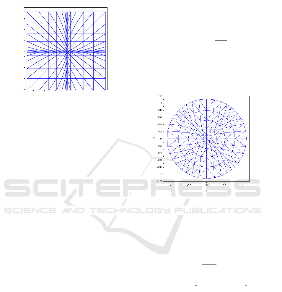
0−2 2−3 −1 1 3
0
−2
2
4
−3
−1
1
3
−3.5
−2.5
−1.5
−0.5
0.5
1.5
2.5
3.5
X
Y
Figure 2: The complex T
F
with F(x, y) = (F
1
(x),F
2
(y))
T
,
where F
1
= F
2
are strictly monotonically increasing contin-
uous functions, linear on each interval [k,k + 1], k ∈Z. The
smaller simplices at the origin lead to long and thin sim-
plices further from the origin.
an underlying basic simplicial complex T and a map-
ping F : R
n
→ R
n
. The relationship between T and
T
F
is that S
F
ν
= co(F(v
0
),F(v
1
),.. ., F(v
n
)) ∈ T
F
, if
and only if S
ν
:= co(v
0
,v
1
,.. ., v
n
) ∈ T . Of course
the mapping F : R
n
→ R
n
must be chosen such that
T
F
is an admissible simplicial complex.
If F is linear, i.e. there exists a matrix F ∈ R
n×n
such that F(x) = Fx, then since
n
∑
i=0
λ
i
F(v
i
) =
n
∑
i=0
λ
i
Fv
i
= F
n
∑
i=0
λ
i
v
i
= F
n
∑
i=0
λ
i
v
i
!
we have
S
F
ν
:= co(F(v
0
),F(v
1
),.. ., F(v
n
))
= co(Fv
0
,Fv
1
,.. ., Fv
n
)
= F co(v
0
,v
1
,.. ., v
n
)
= F(S
ν
)
For many systems, however, one would like to use
smaller simplices close to the origin than further
away. This can be addressed as in e.g. (Marin
´
osson,
2002a; Marin
´
osson, 2002b; Hafstein, 2007) by setting
F(x) = (F
1
(x
1
),F
2
(x
2
),.. ., F
n
(x
n
))
T
, (4)
where the F
i
: R → R are strictly monotonically in-
creasing continuous functions, linear on each interval
[k, k + 1], k ∈ Z. Then F restricted to any z + [0,1]
n
,
z ∈Z
n
, is linear and again S
F
ν
= F(S
ν
) for every sim-
plex S
ν
∈ T . The problem with this approach can be
seen in Figure 2. Smaller simplices at the origin lead
to long and thin simplices further a away.
Further, in many concrete examples is seems nat-
ural that the simplicial complex should be at least
approximately isotropic as viewed from the equilib-
rium at the origin. Neither of these properties can be
achieved by using a linear F or an F as in (4). One
mapping that fulfills these properties is
F(x) = ρ(kxk
∞
) ·
kxk
∞
kxk
2
x, (5)
where ρ : R
+
→ R
+
is a nondecreasing continuous
function. Note that then kF(x)k
2
= ρ(kxk
∞
)kxk
∞
,
i.e. F maps the hypercube [−a,a]
n
bijectively to the
closed hypersphere centered at the origin and with ra-
dius ρ(a)a. See Figure 3 for a picture of T
F
with F
as in (5) and with n = 2.
Figure 3: The complex T
F
with F as in (5) and with ρ(x) =
0.1
√
x.
Such F have been used for example in (Baier et al.,
2012; Bj
¨
ornsson et al., 2014; Baier and Hafstein,
2014; Bj
¨
ornsson et al., 2015). As shown later in this
section some algorithms can be implemented much
more efficiently if a formula for the inverse F
−1
of F
is available. If ρ(x) = sx
q−1
for some s,q > 0, i.e.
F(x) =
skxk
q
∞
kxk
2
x, (6)
then the the inverse of F is given by the formula
F
−1
(x) =
kxk
2
skxk
q
∞
1
q
x =
1
kxk
∞
kxk
2
s
1
q
x. (7)
Note that for F as in (5) the simplex S
F
ν
is not equal to
F(S
ν
). Indeed, F(S
ν
) is not even a simplex, cf. Fig-
ure 4. A contribution of this paper is a fast algorithm
to search for a given x ∈ R
n
a simplex S
F
ν
∈ T
F
such
that x ∈ S
F
ν
, cf. Section 3.2, when the inverse of F is
available but S
F
ν
6= F(S
ν
).
3.1 Implementation of class FT
Let us now discuss the implementation of class FT
modelling T
F
. Its definition is:
Efficient Algorithms for Simplicial Complexes Used in the Computation of Lyapunov Functions for Nonlinear Systems
403
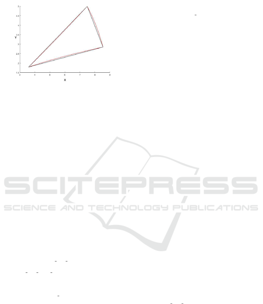
Figure 4: For the simplex S
ν
= co{(2,1)
T
,(3,1)
T
,(3,2)
T
}
and the mapping F(x) = kxk
2
∞
/kxk
2
x the simplex S
F
ν
(black) and the set F(S
ν
) (red/grey).
class FT {
public:
T_std_K *pBC;
function<vec(vec)> pF, ipF;
vec F(vec x);
vec F(ivec x);
vec iF(vec x);
vector<vec> xVer;
vector<mat> XmT;
vector<vec> SCC;
vector<double> SCR;
vector<list<mat>> Fnor;
FT(T_std_K *_pBC, function<vec(vec)> _pF,
function<vec(vec)> _ipF=nullptr);
˜FT();
int InSimpNrSlow(vec x,vec &L);
int InSimpNrFast(vec x,vec &L);
int InSimpNrAppr(vec x);
bool InSimp(vec x,int s,vec &L);
int SVerNr(int s,int i);
vec SVer(int s,int i);
bool CFSS; // default value "true"
};
Let us first discuss the constructor of FT. The class
FT holds a pointer T
std NK *pBC to the under-
lying basic simplicial complex, which is initial-
ized by T std NK * pBC in the constructor. The
mapping F : R
n
→ R
n
that is used to map the
vertices of the basic simplicial complex is stored
as function<vec(vec)> pF, that is initialized by
function<vec(vec)> pF in the constructor, and
can be called with vec F(vec x) and vec F(ivec
x). Their implementation is trivial:
vec F(vec x){
return pF(x);
}
vec F(ivec x){
return pF(conv_to<vec>::from(x));
}
If the inverse mapping F
−1
of F is available, it
can be used to decrease the computational complex-
ity of several algorithms considerably. It is stored
as function<vec(vec)> ipF and is initialized by
function<vec(vec)> ipF in the constructor. If it
is not available we initialize ipF=nullptr. The im-
plementation of the member functions vec iF(vec
x) is analogous to the implementation of vec F(vec
x), just with function<vec(vec)> ipF instead of
function<vec(vec)> pF. To avoid that one delivers
a wrong F
−1
, an error that is bound to happen, it is ac-
tually tested that F
−1
(F(x)) = x for a random sample
in the domain under consideration, i.e. D
T
. Addi-
tionally, we verify F
−1
(0) = 0. This is implemented
as follows in the constructor of FT:
if(ipF!=nullptr){
arma_rng::set_seed_random();
int NrRandVec=1000;
double tol=1e-10;
if(norm(iF(F(zeros<vec>(n))),"inf")>tol){
cerr<<"iF(F(0)) != 0"<<endl;
ipF=nullptr;
}
vec m = F(pBC->Nm);
vec M = F(pBC->Np);
for(int i=0;i<NrRandVec;i++){
vec r=randu<vec>(n);
vec x=r%(M-m)+m;
if(norm(iF(F(x))-x,2)>tol*norm(x,2)){
cerr<<"iF(F(x)) != x for x="<<x.t();
ipF=nullptr;
break;
}
}
}
Note that for vec x and vec y in Armadillo x%y de-
notes element-by-element multiplication, similar to
x.*y in Matlab.
For computational purposes it is advantageous to
store the vertices vector<vec> xVer of T
F
in the
same order as the corresponding integer coordinate
vertices vector<ivec> Ver of T in the basic simpli-
cial complex. This is implemented in the constructor
of FT in the obvious way:
vector<ivec>::iterator p;
for(p=pBC->Ver.begin();p!=pBC->Ver.end();p++){
xVer.push_back(F(*p));
}
The implementation of int FT::SVerNr(int
s,int i) and vec FT::SVer(int s,int i) is
analogous to the implementation of these member
functions in T std NK:
int FT::SVerNr(int s,int i){
return pBC->SVerNr(s,i);
}
vec FT::SVer(int s,int i){
return xVer[SVerNr(s,i)];
}
Further, FT stores for each simplex S
F
ν
the ma-
trix X
−T
ν
, i.e. the inverse of the transpose of the ma-
trix X
ν
, where X
ν
is the so-called shape-matrix of S
F
ν
,
SIMULTECH 2017 - 7th International Conference on Simulation and Modeling Methodologies, Technologies and Applications
404

cf. (Hafstein et al., 2015). The shape-matrix X
ν
of
S
F
ν
= co(v
0
,v
1
,.. ., v
n
) is defined by writing the vec-
tors v
1
−v
0
, v
2
−v
0
, . .., v
n
−v
0
consecutively in its
rows. Note that because the vectors v
0
,v
1
,.. ., v
n
are
affinely independent the matrix X
ν
is invertible. The
matrices X
−T
ν
are stored as vector<mat> XmT in the
same order as the simplices vector<int> pBC->Sim
in the basic simplicial complex. Thus XmT[s] cor-
responds to the simplex pBC->Sim[s]. The rea-
son why we store X
−T
ν
rather than X
−1
ν
or simply
X
ν
is that X
−T
ν
is the most useful form for bool
FT::InSimp(vec x,int s,vec &L).
Further information we want to have ready avail-
able for the simplices S
F
ν
in T
F
are the centers
of their circumscribing hyperspheres and their radii,
stored in vector<vec> SCC and vector<double>
SCR respectively. Again, they are stored in the
same order as the simplices in the basic simplicial
complex, thus SCC[s] is the center and SCR[s] is
the radius of the circumscribing hypersphere of the
simplex pBC->Sim[s]. A formula for the center
c ∈ R
n
of the circumscribing hypersphere of S
F
ν
=
co(v
0
,v
1
,.. ., v
n
) can be derived from the conditions
that
kc −v
i
k
2
2
= r
2
for i = 0,1,. .., n,
where r is the radius of the circumscribed hyper-
sphere. Thus
0 = kc −v
i
k
2
2
−kc −v
0
k
2
2
= −2c
•
(v
i
−v
0
) + kv
i
k
2
2
−kv
0
k
2
2
,
which can be written as
c
•
(v
i
−v
0
) =
1
2
(v
i
−v
0
)
•
(v
i
+ v
0
).
Subtracting v
0
•
(v
i
−v
0
) from both sides delivers
(c −v
0
)
•
(v
i
−v
0
) =
1
2
kv
i
−v
0
k
2
2
,
which gives us a linear equation for c. Set
b = (b
1
,b
2
,.. ., b
n
)
T
with b
i
= kv
i
− v
0
k
2
2
for i =
1,2,. .. ,n. Then
X
ν
(c −v
0
) =
1
2
b
so
c = v
0
+
1
2
X
−1
ν
b.
The radius of the circumscribing hypersphere can
subsequently be computed as
r = kc −v
0
k
2
.
The construction of vector<mat> XmT,
vector<vec> SCC, and vector<double> SCR
is implemented in the constructor of FT as follows.
for(int s=0;s<pBC->Sim.size();s++){
mat XT(n,n);
vec v0=SVer(s,0);
vec b(n);
for(int i=1;i<=n;i++){
XT.col(i-1)=SVer(s,i)-v0;
b(i-1)=pow(norm(XT.col(i-1),2),2);
}
XmT.push_back(XT.i());
vec c=x0+0.5*XmT[s].t()*b;
SCC.push_back(c);
SCR.push_back(norm(c-v0,2));
}
Using the matrices vector<mat> XmT one can
check efficiently if a vector x ∈ R
n
is in a particular
simplex S
F
ν
=Sim[s] or not. Recall that for a simplex
S
F
ν
= co(v
0
,v
1
,v
2
,.. ., v
n
) and a vector x ∈ R
n
, x ∈
S
F
ν
if and only if x can be written as a convex com-
bination of the vertices of the simplex. This means
that there are numbers λ
0
,λ
1
,.. ., λ
n
≥0,
∑
n
i=0
λ
i
= 1,
such that x =
∑
n
i=0
λ
i
v
i
which in turn is equivalent to
x −v
0
=
n
∑
i=1
λ
i
(v
i
−v
0
). (8)
Thus, with L
∗
= (λ
1
,λ
2
,.. ., λ
n
)
T
equation (8) is
equivalent to
X
T
ν
L
∗
= x −v
0
or L
∗
= X
−T
ν
(x −v
0
). (9)
Now x ∈ S
F
ν
if and only if the components of L
∗
are
all nonnegative and sum up to a number ≤1. We then
set λ
0
= 1 −
∑
n
i=0
λ
i
. This is implemented as follows
with L= (λ
0
,λ
1
,.. ., λ
n
)
T
:
bool FT::InSimp(vec x,int s,vec &L){
vec mu=XmT[s]*(x-SVer(s,0));
if(min(mu)>= 0 && sum(mu)<=1){
L(0)=1.0-sum(mu);
L(span(1,n))=mu;
return true;
}
else{
return false;
}
}
Note that vec L contains the barycentric coordinates
of x if it is in Sim[s].
We now come to the discussion of the normals.
Consider a simplex S
ν
= co(v
0
,v
1
,.. ., v
n
) ∈ T
F
.
Another way to characterize the simplex is to define
it as the intersection of (n + 1) half-spaces. These
half-spaces can be constructed by performing the fol-
lowing for each i = 0,1,. .. ,n:
Set y
n
:= v
i
and pick an arbitrary vector y
0
∈
{v
0
,v
1
,.. ., v
n
} \ {v
i
}. Set {y
1
,y
2
,.. ., y
n−1
} =
{v
0
,v
1
,.. ., v
n
}\{y
0
,y
n
} and define the n ×n matrix
Y
i,ν
:= (y
1
−y
0
,y
2
−y
0
,.. ., y
n
−y
0
)
T
.
Efficient Algorithms for Simplicial Complexes Used in the Computation of Lyapunov Functions for Nonlinear Systems
405

Because the vectors y
0
,y
1
,.. ., y
n
are affinely inde-
pendent the matrix Y
i,ν
is non-singular and the equa-
tion
Y
T
i,ν
x = e
n
has a unique solution n
ν
i
= Y
−T
i,ν
e
n
for x. Note that
since
n
ν
i
•
(y
j
−y
0
) = e
T
n
Y
−1
i,ν
(y
j
−y
0
) = e
T
n
e
j
= δ
j,n
,
the vector n
ν
i
is normal to the unique hyperplane con-
taining the vertices {v
0
,v
1
,.. ., v
n
}\{v
i
} of S
F
ν
. Fur-
ther we have for every vector x ∈ S
F
ν
that x is the
convex sum of the vertices v
j
of S
F
ν
and since the y
j
are the same vectors rearranged we have
x =
n
∑
j=0
λ
j
y
j
, 0 ≤ λ
j
≤ 1,
n
∑
j=0
λ
j
= 1.
Hence
n
ν
i
•
(x −y
0
) = n
ν
i
•
n
∑
j=0
λ
j
y
j
−y
0
!
= n
ν
i
•
n
∑
j=1
λ
j
(y
j
−y
0
)
=
n
∑
j=1
λ
j
δ
j,n
= λ
n
≥ 0.
Thus for any i = 0,1,. .. ,n the simplex S
F
ν
is a
subset of the half-space
H
ν
i
:= {x ∈ R
n
: n
ν
i
•
(x −y
0
) ≥ 0}.
Moreover, for each i = 0, 1,.. ., n the vertices
{v
0
,v
1
,.. ., v
n
}\{v
i
} are all in the hyperplane ∂H
ν
i
.
It is easily verified that
S
F
ν
=
n
\
i=0
H
ν
i
. (10)
For our application in constructing linear pro-
gramming problems for the computation of control
Lyapunov functions using the Dini-subdifferential
it is advantageous to store a little more informa-
tion. For each S
F
ν
we consider all its neighbouring
simplices S
F
µ
. For each neighbouring simplex S
F
µ
consider their common face co(f
0
,f
1
,.. ., f
r
). For
each half-space H
µ
k
such that the vertices f
0
,f
1
,.. ., f
r
are all in the hyperplane ∂H
µ
k
we store the corre-
sponding normal n
µ
k
. This can be done by using
the vector<list<int>> T std NK::SimN and
vector<list<vector<int>>> T std NK::Faces
of the basic simplicial complex pointed to by pBC.
First we construct the matrix Y
i,µ
by setting y
0
= f
0
.
The subscript i is arbitrary, except that the i-th vertex
u
i
of S
F
µ
should of course not be the vector f
0
. Then
for every vertex u
k
of S
F
µ
= co(u
0
,u
1
,.. ., u
n
) such
that u
k
/∈ {f
0
,f
1
,.. ., f
r
} we compute n
µ
k
:= Y
−T
i,µ
e
m
,
where m is such that u
k
− y
0
is the m-th line in
Y
i,µ
. Since the vertices in S
F
µ
=Sim[mu] are in some
particular order we just iterate through them and
write the n
µ
k
in the same order in the columns of the
matrix Fnor[nu][mu], where Sim[nu] corresponds
to the simplex S
ν
. This is implemented as follows:
Fnor.resize(pBC->Sim.size());
for(int nu=0;nu<pBC->Sim.size();nu++){
vector<int>::iterator pSN;
vector<vector<int>>::iterator pNP;
pSN=pBC->SimN[nu].begin();
pNP=pBC->Faces[nu].begin();
for(;pSN!=pBC->SimpN[nu].end();pSN++,pNP++){
int mu=*pSN;
vec y0=Vertices[(*pNP)[0]];
int numf=(*pNP).size();
mat Y(n,n),Z(n,n-numf+1,fill::zeros);
int j=0,k=0;
for(int i=0;i<=n;i++){
if(SVerNr(mu,i)!=(*pNP)[0]){
Y.col(j)=SVer(mu,i)-y0;
if(binary_search((*pNP).begin(),
(*pNP).end(),SVerNr(mu,i))==false){
// vertex i of Sim[mu] is not in
// the face
Z(j,k++)=1.0;
}
j++;
}
}
Fnor[nu].push_back(solve(Y.t(),Z));
}
}
3.2 Fast Search for S
F
ν
such that x ∈ S
F
ν
Given an x ∈ R
n
one is often interested in finding an
S
F
ν
∈ T
F
such that x ∈ S
F
ν
. Additionally, one of-
ten then needs the barycentric coordinates of x in S
ν
,
i.e. the λ
i
such that x =
∑
n
i=0
λ
i
v
i
is the convex com-
bination of the vertices v
i
of S
F
ν
. Without any ad-
ditional information one must rely on linear search,
implemented as:
int FT::InSimpNrSlow(vec x,vec &L){
for(int s=0;s<pBC->Sim.size();s++){
if(InSimp(x,s,L)==true){
return s;
}
}
return -1;
}
Note that the vec &L corresponds to the vector
(λ
0
,λ
1
,.. ., λ
n
)
T
and if a simplex containing x is not
found the return value is set to the impossible value
−1.
If a formula for the inverse mapping F
−1
of F is
available we can do much better. For some applica-
tion, e.g. when plotting a computed Lyapunov func-
SIMULTECH 2017 - 7th International Conference on Simulation and Modeling Methodologies, Technologies and Applications
406

tion, it is sometimes enough to get a simplex S
F
ν
such
that x is close to S
F
ν
. This can be done by finding a
simplex S
ν
in T , such that y := F
−1
(x) ∈ S
ν
. Recall
the such an S
ν
can be computed very efficiently in
the member function T std NK::InSimpNr(vec x)
as described in (Hafstein, 2013). This is implemented
as
int FT::InSimpNrAppr(vec x){
assert(ipF!=nullptr);
return pBC->InSimpNr(iF(x));
}
For many applications this is, however, not sufficient.
An example is when a linear programming problem
for discrete-time dynamical systems is constructed,
cf. (Giesl and Hafstein, 2014a; Hafstein et al., 2014;
Li et al., 2015). Then a simplex S
F
ν
such that x ∈ S
F
ν
and the barycentric coordinates of x are necessary.
If one can be sure that x /∈ D
F
T
:=
S
S
ν
∈T
S
F
ν
follows from F
−1
(x) /∈ D
T
, one can set the mem-
ber variable bool CFSS (careful simplex search),
whose default value is true, equal to false. Note
that this holds true in the important case that F
and F
−1
are as in (6) and (7) and N
p
= −N
m
=
(N,N, .. .,N)
T
for a positive integer N in T = T
std
N,K
(Np=ivec(n).fill(N) and Nm=-Np in the basic com-
plex pointed to by pBC). The reason is that then F
maps the hypercube D
T
= {x ∈R
n
: kxk
∞
≤N} onto
the closed hypersphere S
R
⊂ R
n
centered at the ori-
gin and with radius R = sN
q
. Since S
R
is convex
it clearly contains D
F
T
and consequently F
−1
(D
F
T
) ⊂
F
−1
(S
R
) = D
T
.
The idea behind the fast search for a simplex
S
F
ν
∈T
F
such that x ∈S
F
ν
is as follows: Given x ∈R
n
compute a simplex S
ν
∈ T such that F
−1
(x) ∈ S
ν
.
If x ∈ S
F
ν
we are finished. If not check if x ∈ S
F
µ
for all neighbouring simplices S
F
µ
of S
F
ν
. If an S
F
µ
is
found such that x ∈S
F
µ
we are finished. If not check if
x ∈ S
F
ξ
for all neighbouring simplices S
F
ξ
of the sim-
plices S
F
µ
that have not already been checked. Repeat
this as necessary. The implementation is as follows:
int FT::InSimpNrFast(vec x,vec &L){
int s=InSimpNrAppr(vec x)
if(s==-1){
if(CFSS==true){ // might be in complex
s=InSimpNrSlow(x,L);
}
return s;
}
if(InSimp(x,s,L)==true){
return s;
}
list<int> TC, CH, CN;
// TC = To Check
// CH = already CHecked
// CN = Check Next
TC=pBC->SimN[s];
list<int>::iterator p;
for(p=TC.begin();p!=TC.end();p++){
if(InSimp(x,*p,L)==true){
return *p;
}
}
// initialize the main loop
CH.push_back(s);
TC.push_back(s);
int MaxSweeps=3;
while(MaxSweeps--){
CN.clear();
for(p=TC.begin();p!=TC.end();p++){
list<int> A2CN=pBC->SimN[*p];
CN.insert(CN.end(),
A2CN.begin(),A2CN.end());
}
CN.sort();
CN.unique();
TC.clear();
set_difference(CN.begin(),CN.end(),
CH.begin(),CH.end(),back_inserter(TC));
if(TC.empty()==true){
return -1;
}
for(p=TC.begin();p!=TC.end();p++){
if(InSimp(x,*p,L)==true){
return *p;
}
}
CH.insert(CH.end(),TC.begin(),TC.end());
CH.sort();
}
return InSimpNrSlow(x,L);
}
We have two comments on this algorithm. First, if
the main loop is used to search through the whole
complex, then it is considerably slower than a lin-
ear search by FT::InSimpNrSlow(x,L). Thus, the
implementation uses the parameter int MaxSweeps
to decide when to give up on searching for neigh-
bours and just do a linear search through the whole
complex. Its appropriate value will depend on the
kind of the problem at hand to be solved. We used
MaxSweeps=3 which worked quite well for our exam-
ples. Second, instead of using all neighbours one can
instead use only neighbours with common faces that
are maximal, i.e. (n −1)-simplices (n common ver-
tices). This actually turned out to be faster in many
cases, but since the essential idea is the same we do
not discuss it further here.
To give an idea of the improvement in running
times in comparison to linear search see Table 1. In all
runs we generated 10,000 uniformly distributed ran-
dom points x in the hypercube [−N,N]
n
and searched
for a simplex S
F
ν
such that F(x) ∈ S
F
ν
.
As an example, if one wants to generate a linear
programming problem to compute a Lyapunov func-
Efficient Algorithms for Simplicial Complexes Used in the Computation of Lyapunov Functions for Nonlinear Systems
407

Table 1: The running times for the search of a simplex S
F
ν
∈
T
F
such that x ∈T
F
for a random sample of 10,000 points
x. The mapping F was as in (6) with s = 0.1 and q = 1.5.
n is the dimension and N and K are the parameters of the
complex T = T
std
N,K
. [neigh.] is the proportion of simplices
such that we do not get a direct hit, i.e. x /∈ S
F
ν
although
F
−1
(x) ∈ S
ν
. [lin.] is the time needed for linear search
and [opt.] is the time needed for the new algorithm. The
algorithms were run on a PC machine: i4790k@4600MHz
with 32GB RAM.
n N K neig.[%] lin. [sec] opt.[sec]
2 20 0 1.1 0.699 0.033
2 20 5 0.87 0.670 0.066
2 50 0 0.44 4.445 0.039
2 50 5 0.39 4.417 0.046
2 50 10 0.35 4.313 0.079
2 100 0 0.24 21.61 0.041
2 100 5 0.24 21.98 0.042
2 200 0 0.14 90.50 0.046
2 200 10 0.14 90.29 0.051
3 15 0 2.28 49.33 0.169
3 15 5 2.6 48.93 0.862
3 25 0 1.67 245.8 0.218
3 25 5 1.60 229.6 0.376
4 10 0 6.40 1154 10.12
tion for a time-discrete system x
k+1
= g(x
k
) using the
simplicial complex in the table with n = 3, N = 25,
and K = 0, which has 51
3
= 132,651 vertices and
3! ·50
3
= 750, 000 simplices, the running time for the
search for simplices S
F
ν
such that g(x) ∈ S
F
ν
for all
the vertices x of the complex is reduced from 54 min-
utes to less than 3 seconds using the new algorithm!
4 SUMMARY
We described the efficient implementation of simpli-
cial complexes for the computation of Lyapunov func-
tions for nonlinear systems. This paper is a logical
sequel to the papers (Hafstein, 2013; Giesl and Haf-
stein, 2014b; Bj
¨
ornsson et al., 2015) and explains
how to adapt algorithms for the simplicial complex
to compute Lyapunov functions for time-discrete sys-
tems and control systems. An additional bonus is that
some of the algorithms can be used for different com-
putational methods that depend on conic partitions of
the state-space as discussed in Section 2.1.
The probably best know method for computing
Lyapunov functions for rather general nonlinear sys-
tems is the so-called SOS (sum-of-squares) method,
cf. e.g. (Parrilo, 2000; Peet and Papachristodoulou,
2012; Peet, 2009; Anderson and Papachristodoulou,
2015). A reason for this is definitely that its im-
plementation is not too difficult and that a well
documented Matlab library, SOSTOOLS, is available
(Papachristodoulou et al., 2013). It is the hope
of the author that this paper brings the techniques
necessary for the efficient implementation of the CPA
method to compute Lyapunov functions for nonlinear
systems closer to interested researchers. It definitely
is an important milestone in the development of an
easy-to-use C++ program for such computations for
very general nonlinear systems.
ACKNOWLEDGEMENT
The author’s research is supported by the Icelandic
Research Fund (Rann
´
ıs) ‘Complete Lyapunov func-
tions: Efficient numerical computation’ (163074-052)
and ‘Lyapunov Methods and Stochastic Stability’
(152429-051), which is gratefully acknowledged.
REFERENCES
Ambrosino, R. and Garone, E. (2012). Robust stability of
linear uncertain systems through piecewise quadratic
Lyapunov functions defined over conical partitions. In
Proceedings of the 51st IEEE Conference on Decision
and Control, pages 2872–2877, Maui (HI), USA.
Anderson, J. and Papachristodoulou, A. (2015). Advances
in computational Lyapunov analysis using sum-of-
squares programming. Discrete Contin. Dyn. Syst. Ser.
B, 20(8):2361–2381.
Baier, R., Gr
¨
une, L., and Hafstein, S. (2012). Linear pro-
gramming based Lyapunov function computation for
differential inclusions. Discrete Contin. Dyn. Syst. Ser.
B, 17(1):33–56.
Baier, R. and Hafstein, S. (2014). Numerical computation
of Control Lyapunov Functions in the sense of gen-
eralized gradients. In Proceedings of the 21st Inter-
national Symposium on Mathematical Theory of Net-
works and Systems (MTNS), pages 1173–1180 (no.
0232), Groningen, The Netherlands.
Bj
¨
ornsson, J., Giesl, P., Hafstein, S., Kellett, C., and Li,
H. (2014). Computation of continuous and piecewise
affine Lyapunov functions by numerical approxima-
tions of the Massera construction. In Proceedings
of the CDC, 53rd IEEE Conference on Decision and
Control, Los Angeles (CA), USA.
Bj
¨
ornsson, J., Gudmundsson, S., and Hafstein, S. (2015).
Class library in C++ to compute Lyapunov functions
for nonlinear systems. In Proceedings of MICNON,
1st Conference on Modelling, Identification and Con-
trol of Nonlinear Systems, number 0155, pages 788–
793.
Branicky, M. (1998). Multiple Lyapunov functions and
other analysis tools for switched and hybrid systems.
IEEE Trans, 43(4):475–482.
SIMULTECH 2017 - 7th International Conference on Simulation and Modeling Methodologies, Technologies and Applications
408

Clarke, F. (1990). Optimization and Nonsmooth Analysis.
Classics in Applied Mathematics. SIAM.
Giesl, P. and Hafstein, S. (2014a). Computation of Lya-
punov functions for nonlinear discrete systems by lin-
ear programming. J. Difference Equ. Appl., 20:610–
640.
Giesl, P. and Hafstein, S. (2014b). Implementation of a fan-
like triangulation for the CPA method to compute Lya-
punov functions. In Proceedings of the 2014 Ameri-
can Control Conference, pages 2989–2994 (no. 0202),
Portland (OR), USA.
Giesl, P. and Hafstein, S. (2014c). Revised CPA method to
compute Lyapunov functions for nonlinear systems. J.
Math. Anal. Appl., 410:292–306.
Hafstein, S. (2007). An algorithm for constructing Lya-
punov functions, volume 8 of Monograph. Electron.
J. Diff. Eqns.
Hafstein, S. (2013). Implementation of simplicial com-
plexes for CPA functions in C++11 using the ar-
madillo linear algebra library. In Proceedings of SI-
MULTECH, pages 49–57, Reykjavik, Iceland.
Hafstein, S., Kellett, C., and Li, H. (2014). Computation
of Lyapunov functions for discrete-time systems using
the Yoshizawa construction. In Proceedings of CDC.
Hafstein, S., Kellett, C., and Li, H. (2015). Computing con-
tinuous and piecewise affine lyapunov functions for
nonlinear systems . Journal of Computational Dynam-
ics, 2(2):227 – 246.
Johansson, M. (1999). Piecewise Linear Control Systems.
PhD thesis: Lund University, Sweden.
Johansson, M. and Rantzer, A. (1998). Computation of
piecewise quadratic Lyapunov functions for hybrid
systems. IEEE Trans. Automat. Control, 43(4):555–
559.
Julian, P. (1999). A High Level Canonical Piecewise Lin-
ear Representation: Theory and Applications. PhD
thesis: Universidad Nacional del Sur, Bahia Blanca,
Argentina.
Julian, P., Guivant, J., and Desages, A. (1999). A
parametrization of piecewise linear Lyapunov func-
tions via linear programming. Int. J. Control, 72(7-
8):702–715.
Lazar, M. (2010). On infinity norms as Lyapunov func-
tions: Alternative necessary and sufficient conditions.
In Proceedings of the 49th IEEE Conference on Deci-
sion and Control, pages 5936–5942, Atlanta, USA.
Lazar, M. and Doban, A. (2011). On infinity norms as Lya-
punov functions for continuous-time dynamical sys-
tems. In Proceedings of the 50th IEEE Conference
on Decision and Control, pages 7567–7572, Orlando
(Florida), USA.
Lazar, M., Doban, A., and Athanasopoulos, N. (2013). On
stability analysis of discrete-time homogeneous dy-
namics. In Proceedings of the 17th International
Conference on systems theory, control and computing,
pages 297–305, Sinaia, Romania.
Lazar, M. and Joki
´
c, A. (2010). On infinity norms as Lya-
punov functions for piecewise affine systems. In Pro-
ceedings of the Hybrid Systems: Computation and
Control conference, pages 131–141, Stockholm, Swe-
den.
Li, H., Hafstein, S., and Kellett, C. (2015). Computation of
continuous and piecewise affine Lyapunov functions
for discrete-time systems. J. Difference Equ. Appl.,
21(6):486–511.
Marin
´
osson, S. (2002a). Lyapunov function construction
for ordinary differential equations with linear pro-
gramming. Dynamical Systems: An International
Journal, 17:137–150.
Marin
´
osson, S. (2002b). Stability Analysis of Nonlin-
ear Systems with Linear Programming: A Lyapunov
Functions Based Approach. PhD thesis: Gerhard-
Mercator-University Duisburg, Duisburg, Germany.
Ohta, Y. (2001). On the construction of piecewise lin-
ear Lyapunov functions. In Proceedings of the 40th
IEEE Conference on Decision and Control., volume 3,
pages 2173–2178.
Ohta, Y. and Tsuji, M. (2003). A generalization of piece-
wise linear Lyapunov functions. In Proceedings of the
42nd IEEE Conference on Decision and Control., vol-
ume 5, pages 5091–5096.
Papachristodoulou, A., Anderson, J., Valmorbida, G.,
Pranja, S., Seiler, P., and Parrilo, P. (2013). SOS-
TOOLS: Sum of Squares Optimization Toolbox for
MATLAB. User’s guide. Version 3.00 edition.
Parrilo, P. (2000). Structured Semidefinite Programs and
Semialgebraic Geometry Methods in Robustness and
Optimiza. PhD thesis: California Institute of Technol-
ogy Pasadena, California.
Peet, M. (2009). Exponentially stable nonlinear systems
have polynomial Lyapunov functions on bounded re-
gions. IEEE Trans. Automat. Control, 54(5):979 –
987.
Peet, M. and Papachristodoulou, A. (2012). A con-
verse sum of squares Lyapunov result with a degree
bound. IEEE Transactions on Automatic Control,
57(9):2281–2293.
Polanski, A. (1997). Lyapunov functions construction by
linear programming. IEEE Trans. Automat. Control,
42:1113–1116.
Polanski, A. (2000). On absolute stability analysis by poly-
hedral Lyapunov functions. Automatica, 36:573–578.
Sanderson, C. (2010.). Armadillo: An open source C++
linear algebra library for fast prototyping and com-
putationally intensive experiments. Technical report,
NICTA.
Yfoulis, C. and Shorten, R. (2004). A numerical technique
for the stability analysis of linear switched systems.
Int. J. Control, 77(11):1019–1039.
Efficient Algorithms for Simplicial Complexes Used in the Computation of Lyapunov Functions for Nonlinear Systems
409
