Fault Estimation using a Takagi-Sugeno Interval Observer: Application

to a PEM Fuel Cell

C. Mart

ınez Garc

ıa

, V. Puig

and C. Astorga Zaragoza

Centro Nacional de Investigaci

on y Desarrollo Tecnol

ogico, Cuernavaca, Morelos, Mexico

Universitat Polit

ecnica de Catalunya, Departament of Automatic Control, Rambla de Sant Nebridi 10, Terrassa, Spain

Keywords:

Takagi-Sugeno System, Interval Observer, Fault Estimation, PEM Fuel Cell.

Abstract:

Fault estimation plays an important role in the fault diagnosis system since provides information about the fault

magnitude and temporal evolution. In this paper, we present an approach that allows to obtain a simultaneous

estimation of the fault, state and associated uncertainty intervals of a uncertain Takagi-Sugeno (TS) system.

The fault estimation is obtained using a TS interval observer augmenting the system state with the fault and

considering the system uncertainty in a bounded context. A set of Linear Matrix Inequalities (LMIs) have

been derived to design the TS interval observer. With the purpose of illustrating the performance of TS

interval observer for fault and state estimation, a case study based on a Proton Exchange Membrane (PEM)

fuel cell is used.

1 INTRODUCTION

Fault diagnosis involves the fault detection and iso-

lation but also the fault estimation. The fault de-

tection and isolation tasks determine the fault pres-

ence in the system (Zhang and Jiang, 2008) (Hwang

et al., 2010) (Samy et al., 2011), but not the mag-

nitude. The goal of fault estimation is to provide

the size of the fault and its time evolution (Blanke

et al., 2006). The fault estimation task is very im-

portant for several applications, especially when an

active fault-tolerant control (FTC) strategy is imple-

mented (Mahmoud et al., 2003) (Noura et al., 2009)

(Witczak, 2014). An example of the application of

the fault estimation is to determine the size of the

leaks in a pipe system with the aim of quantifying

the losses (Brune and F, 2001). There are several ap-

proaches for addressing the problem of diagnosis of

non-linear systems (Witczak, 2007). In this paper, we

can consider that the non-linear model of the system

to be monitored can be represented by Takagi-Sugeno

(TS) model. TS models were introduced by (Takagi

and Sugeno, 1985), and allow describing a nonlin-

ear system as the interpolation of linear models by

means of membership functions, that come from a set

of fuzzy rules. Different observer design techniques

have been developed for TS systems (Guerra et al.,

2015) (Aouaouda et al., 2014) (Ichalal et al., 2010)

(Zhang et al., 2009).

The presence of uncertainties (unknown parame-

ters, disturbances and/or noise) in the system, compli-

cates the estimation using standard (non-robust) ob-

servers. Interval observers can be used to take into

account the uncertainty using the set-membership ap-

proach (Puig, 2010). The interval observer consid-

ers the disturbances, noise and model parameters in

a bounded way, evaluating the set of admissible val-

ues (interval) for the state vector of each time instant

(Eﬁmov et al., 2013b). So far, interval observers have

been proposed for the state estimation (Eﬁmov et al.,

2013b) and fault detection of nonlinear and LPV sys-

tems (Eﬁmov et al., 2013a). As explained in (Rassi

et al., 2010), the general idea is to build two ob-

servers, which respectively estimate the lower and up-

per bound of the state vector assuming the system is

cooperative. As the original nonlinear system is not

cooperative, the observer gain is designed such that

the observation error dynamics becomes cooperative.

The inclusion of uncertainty in the model parameters

in case of an interval observer allows robust fault de-

tection. In (Rotondo et al., 2016), this idea has been

used for the fault diagnosis of proton exchange mem-

brane (PEM) fuel cells using a TS interval observer

approach. The TS interval observer design is used for

the state estimation of TS uncertain systems. Fault

diagnosis is addressed using a bank observers where

each observer can be made sensitive to different sub-

set of faults.

García, C., Puig, V. and Zaragoza, C.

Fault Estimation using a Takagi-Sugeno Interval Observer: Application to a PEM Fuel Cell.

DOI: 10.5220/0006431206130620

In Proceedings of the 14th International Conference on Informatics in Control, Automation and Robotics (ICINCO 2017) - Volume 1, pages 613-620

ISBN: 978-989-758-263-9

613

The novelty of this paper is to present a fault esti-

mation scheme based on a TS interval observer. This

estimator obtain the simultaneous state and fault esti-

mation without making use of the fault detection and

isolation modules. Moreover, an interval of the fault

magnitude is provided which has not yet been pro-

posed for fault estimation in TS systems. The design

of the TS interval observer is addressed with the Lya-

punov approach leading to a set of LMIs, that can be

efﬁciently solved using available solvers as YALMIP

ofberg, 2004). The performance of the TS interval

observer for the fault and state estimation is assessed

using a case study based on a proton exchange mem-

brane (PEM) fuel cell.

The structure of the paper is the following: In the

Section 2, the uncertain TS system is presented. In

the Section 3, the formulation of the interval observer

design is presented. The proposed PEM fuel cell case

study is presented in Section 4, while the results of the

application of the proposed approach are presented.

Finally, Section 5 presents conclusions of this work.

2 PROBLEM SETUP

2.1 Takagi-Sugeno Uncertain Model

The uncertain TS model of the system to be monitored

is expressed in discrete-time including parametric un-

certainty as follows:

Rule i : If ρ

(k) is M

and ··· and ρ

(k) is M

Then











(k + 1) = (A

+ ∆A

(k) + B

u(k)

(k) + Dd(k)

(k) = Cx

(k) + E

(k) + Gv(k)

(1)

where i = {1, 2, · · · , r} and r is the number of rules as-

sociated to the different submodels, x(k) ∈ R

is the

state vector, u(k) ∈ R

is the input vector, y(k) ∈ R

is the measured output vector, d(k) ∈ R

is the ex-

ogenous disturbance, v(k) ∈ R

is the measurement

noise, M denote fuzzy sets and ρ

(k), · · · , ρ

(k) are

the premise variables. E

is fault distribution matrix

of actuator faults f

(k). Analogously, E

is the fault

distribution matrix of sensor faults f

(k). Combining

the local subsystems (1) considering the level of sat-

isfaction of each rule, the following model for the TS

system can be obtained:

x(k + 1) =

∑

i=1

(ρ(k))(A

+ ∆A

x(k) + B

u(k))

+ E

(k) + Dd(k)

y(k) = Cx(k) + E

(k) + Gv(k)

(2)

where ρ(k) = [ρ

(k), · · · , ρ

(k)]

is the vector con-

taining the premise variables, η

(ρ(k)) and ξ

(ρ(k))

are deﬁned as follows:

(ρ(k)) =

∏

j=1

i j

(ρ

(k))

(3)

(ρ(k)) =

(ρ(k))

∑

i=1

(ρ(k))

(4)

where η

(ρ(k))(product of the membership functions

that correspond to the fuzzy sets of a i-th rule) is the

membership grade of ρ

(k) in η

i j

and ξ

(ρ(k)) is the

normalized membership function deﬁned as:











∑

i=1

(ρ(k)) = 1

(ρ(k)) ≥ 0, i = {1,2,··· ,r}.

(5)

The matrices A

∈ R

×n

, B

∈ R

×n

and C ∈ R

×n

contain the system nominal parameters, ∆A

∈ R

×n

represent the parametric uncertainty that is assumed

to be not known but bounded ∆A

≤ ∆A

. Dis-

turbances d(k) and noise v(k) (assuming that V (k) is

the upper bound from measurement noise) are also

considered bounded, as follows:

d(k) ≤ d(k) ≤ d(k) (6)

v(k)

≤ V (k) (7)

2.2 Fault Estimation Scheme

2.2.1 Problem Formulation

The proposed fault estimation is based on designing

a TS interval observer for the uncertain system (2)

considering an augmented state vector that considers

faults in sensors ( f

(k)) and actuators ( f

(k)) as fol-

lows:

x(k) =



x(k) f

(k) f

(k)



(8)

The TS interval observer will provide an interval esti-

mation of the augmented stated

x(k) ≤

x(k) (9)

ICINCO 2017 - 14th International Conference on Informatics in Control, Automation and Robotics

614

i.e., of the states and faults:

ˆx(k) ≤ x(k) ≤ ˆx(k) (10)

(k) ≤ f

(k) ≤

(k) (11)

(k) ≤ f

(k) ≤

(k) (12)

When creating the augmented model, it is considered

that the actuator fault (11) is modelled as follows:

(k + 1) = f

(k) + w

(k) (13)

where w

(k) ∈ R

considers the actuator fault varia-

tions that assumed to be bounded

(k) ≤ w

(k) (14)

Similarly, the sensor fault f

(k) ∈ R

is modelled as

follows:

(k + 1) = f

(k) + w

(k) (15)

where w

(k) ∈ R

considers the sensor fault varia-

tions that assumed to be bounded

(k) ≤ w

(k) (16)

(k) and w

(k) allowing to consider non-constant

faults.

The variations of the faults (w

(k) and w

(k)) are

taken into account altogether with the system distur-

bance d(k) by means of an augmented disturbance

considered for the TS interval observer design as fol-

lows:

d(k) =



d(k) w

(k) w

(k)



(17)

Considering the fault models (13) and (15), the aug-

mented model of the system considered for the design

the TS interval observer can be expressed in the fol-

lowing form:

x(k + 1) =

∑

i=1

(ρ(k))((

+ ∆

)

x(k) +

u(k))

d(k)

y(k) =

x(k) + Gv(k)

(18)

with:





0 I 0

0 0 I













x(k) =





x(k)

(k)





∆





∆A

0 0

0 0 0





C =



C 0 E



D =









where

∈ R

×n

are the matrices that contain

the matrices of distribution of f

(k) and f

(k).

The interval observer for TS system (18), follows the

Luenberger form (according to (Rotondo et al., 2016)

and (Eﬁmov et al., 2013b)):

x(k + 1) =

∑

i=1

(ρ(k))(

−

x(k) +

u(k) + (

∆A

(k) −

∆A

−

(k) −

∆A

−

(k) +

∆A

−

(k))

y(k) −



V (k)E

d(k)

x(k + 1) =

∑

i=1

(ρ(k))(

−

x(k) +

u(k) + (

∆A

(k) −

∆A

−

(k) −

∆A

−

(k) +

∆A

−

(k))

y(k) +



V (k)E

d(k)

(19)

with:





i,x

i, f









i,x

i, f





x(k) =







ˆx

(k)

i, f

(k)

i, f

(k)







x(k) =

ˆx

(k)

i, f

(k)

i, f

(k)

where

∈ R

×n

and

∈ R

×n

are the

observer gains to be designed,

∆A

= max

∆A

−

∆A

−

∆A

= max

∆A

−

∆A

−

∆A

= max

−

= max

−

x and, ﬁnally E

∈

×1

is the column vector with elements equal to 1.

d(k) and

d(k) are the bounds from (17). The output

interval estimation of y(k) can be obtained as follows:

y =

x and

y =

To design the TS interval observer for the sys-

tem (2) with the augmented state vector including the

faults (13) and (15) should be observable. Observabil-

ity of the TS uncertain system (2) can be assessed us-

ing the approach proposed in (Ho et al., 2013). If the

following, it is assumed that this observability condi-

tion for the augmented system (18) is satisﬁed.

2.2.2 Integration with FDI

The proposed fault estimation scheme could be inte-

grated with a FDI scheme as the one proposed in (Ro-

tondo et al., 2016) and only activated once the fault

has been detected and isolated. In particular, a bank

of a bank of n

dedicated observers where each ob-

server has been designed to estimate only one fault

Fault Estimation using a Takagi-Sugeno Interval Observer: Application to a PEM Fuel Cell

615

Figure 1: Integration with FDI using a bank of observers.

will be designed. Then, the TS interval observer that

considers as additional state the fault that has been

detected and isolated will be used for estimating the

fault. Alternatively, the fault estimation scheme can

be integrated with a bank of n

dedicated observers

where each observer has been designed to be sensi-

tive to only one fault (using as e.g., an unknown input

observer approach (Blanke et al., 2006)), as shown in

Fig. 1. In this second case, the following fault detec-

tion and isolation logic can be used: While the fault

estimation intervals provided by all the observers in

the bank satisfy

0 ∈ [

] i = 1,··· ,n

no fault is detected. Otherwise, when some of the ob-

servers provides a fault estimation interval satisfying

0 /∈ [

]

it means that the fault f

has been ocurred, being the

fault magnitude bounded by [

]

3 TAKAGI-SUGENO INTERVAL

OBSERVER DESIGN

To design a TS interval observer of the form (19) that

ensures (9), (and therefore (10), (11) and (12)) with

acceptable performance speciﬁed by means of an LMI

region, the following theorem is introduced.

Theorem 1. Given positive scalars ε

> 0, ε

> 0, a

TS interval observer (19) with performance deﬁned

with an LMI region deﬁned by two vertical strips (h

and h

) and a disk (r and q are the radius and center)

can be obtained, if there exist matrices P = P

> 0,

Q > 0 and

∈ R

×2n

∈ R

×2n

that

satisfy the following inequalities for i = {1,2,··· ,r}:





1+ε

−W

1+ε

(PD

−W

ϒ)

P − Q − λη

1+ε

0 λI

− τP





≥ 0

(20)





−W

ϒ ≥ 0 (21)





−rP ∗

qP + P





−W

ϒ −rP





< 0 (22)





P + P





+ 2h

P < 0 (23)





P + P





+ 2h

P > 0 (24)

with W

, λ > 0, τ = 1 + ε

+ (1 + ε

)

−1

∆A

ϒ =



C 0



Proof: The theorem can be easily proved adapting

the results of (Eﬁmov et al., 2013b) for LPV systems

and (Chilali and Gahinet, 1996) for pole placement in

one the LMI region.

Then, the gains of the interval observer (19) are

obtained after solving the inequalities (20), (21), (22),

(23) and (24)) as follows

= P

−1

and

= P

−1

(25)

with i = {1,2,··· ,r}.

4 CASE STUDY

4.1 Fuel Cell System

Fuel cells have been considered as alternative energy

sources for the future with potential application to

several areas: transport (buses, trucks, trains, etc),

military applications (portable soldier power), auxil-

iary power units, and electricity generation provide

electricity (and sometimes heat) (Wee, 2007). Pro-

ton exchange membrane fuel cells (PEMFC) are elec-

tromechanical devices in which the energy of a re-

action between a fuel, the hydrogen, and oxidant,

the oxygen, is directly and continuously converted

into electrical energy, obtaining water as a subprod-

uct (Pukrushpan et al., 2004). In the literature, we can

ICINCO 2017 - 14th International Conference on Informatics in Control, Automation and Robotics

616

ﬁnd works dealing with PEMFC, considering durabil-

ity, optimal control, model predictive control, fault di-

agnosis and different approaches for fuell cell model-

ing (electric equivalent model, state space model,etc)

(Rotondo et al., 2016).

The nonlinear model of the PEMFC (Pukrush-

pan et al., 2004), can be derivate by four subsys-

tems: compressor, supply manifold, cathode plus re-

turn manifold and anode. For illustrating purposes

and because of space limitations, the scheme pro-

posed in this paper only the compressor subsystem is

used.

4.2 Compressor System

The model of the compressor is described by means

of the following equation:

= (−

)ω

(

−

amb

)

(26)

where ω

is the compressor speed, K

is the motor

electric constant, J

is the compressor and motor in-

ertia, R

is the compressor motor circuit resistance,

is the air heat capacity at constant pressure, T

amb

is the ambient temperature and η

is the compressor

efﬁciency V

is the voltage,

1,2,3

are function of

the stack current I

. For assessing the nonlinear

compressor model the values and parameters of the

Table 1 and 2 are considered.

The model (26) can be rewritten of the form (2)

with the nonlinear sector approach, considering the

following that ρ(k) = I

(k) and the state space matri-

ces are:

A(ρ(k)) = (−

)

B(ρ(k)) =

(

−

amb

)

where ω

is the state, V

is the input, I

is the

variable parameter. The dimensions of the matrices

are A(ρ(k)) ∈ R

1×1

and B(ρ(k)) ∈ R

1×1

The vertices models are scheduled under the

following:

ρ(k) =

(k)−I

stmin

stmax

−I

stmin

and ρ(k) =

stmax

−I

(k)

stmax

−I

stmin

Then, in order to obtain the results of the scheme

proposed is considered that the stack current is in the

range I

∈



100,300



mA. Then, using a sequence

of steps of 10 mA a set of 21 possible operating

points are obtained. The systems is discretized with a

sampling time T

= 0.01s.

Table 1: Parameters of the nonlinear model of a compressor.

Symbol Value

0.0153 V /(rad/s)

5 × 10

−5

kg· m

0.816 Ω

1004 J/(kg· K)

amb

298 K

0.9

Table 2: Variables in the nonlinear model of a compressor.

Approximate variables

≈ 0.777217

≈ 0.275641 ·10

−3

− 0.340993·10

−3

≈ 0.001375I

− 0.023710

≈ −0.000426 ·10

−3

+ 0.213459·10

−3

4.3 Actuator Fault Estimation

For the actuator fault estimation, the following

dedicated observer is used:











x(k + 1) =

∑

i=1

(ρ(k))(

−

[C 0])

x(k) +

u(k)

∆A

(k) −

∆A

−

(k) −

∆A

−

(k)

∆A

−

(k) +

y(k) −



V (k)E

d(k)

x(k + 1) =

∑

i=1

(ρ(k))(

−

[C 0])

x(k) +

u(k)

∆A

(k) −

∆A

−

(k) −

∆A

−

(k) +

∆A

−

(k) +

y(k) +



V (k)E

d(k)

(27)

with:



0 I









i,x

i, f





i,x

i, f



x(k) =



ˆx(k)

i, f

(k)



x(k) =

x(k)

i, f

(k)

∆A



∆A

0 0



∆A



∆A

0 0



∆A

−



∆A

−

0 0



∆A

−



∆A

−

0 0



D =





The observer gains are placed in a LMI region,

deﬁned as the intersection of a disk sector with

r = 1, q = 0 and two vertical strips: h

= −0.11 and

= −0.9.

Fault Estimation using a Takagi-Sugeno Interval Observer: Application to a PEM Fuel Cell

617

To assess the performance of fault estimation

provided by the TS interval observer, two type of

faults are considered (abrupt fault and incipient fault).

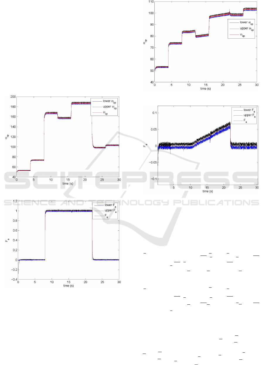
Case 1.- Abrupt Fault

With the aim of showing the estimator performance in

case of an actuator fault, an abrupt change of 8 to 22

sec is made. Figure 2 shows that although there exists

a fault, the observer is able to estimate ω

Figure 3 presents the fault estimation ( f

) where

the estimator is slow when the fault occurs but after

a transient it can provide an interval for the fault esti-

mation.

Figure 2: Estimation of ω

Figure 3: Estimation of f

Case 2.- Incipient Fault

Considering an incipient fault scenario, we can ob-

serve that the observer is able to estimate this type of

fault, Figure 4 shows the state estimation ω

while

Figure 5 illustrates the fault estimation. From these

two ﬁgures, it can be seen that the observer (27) is

able to estimate adequately the fault and the state.

Figure 4: Estimation of ω

Figure 5: Estimation of f

4.4 Sensor Fault Estimation

For the sensor fault estimation, the following TS

interval observer is used:











x(k + 1) =

∑

i=1

(ρ(k))(

−

[C E

])

x(k) +

u(k)

∆A

(k) −

∆A

−

(k) −

∆A

−

(k) +

∆A

−

(k) +

y(k) −



V (k)E

d(k)

x(k + 1) =

∑

i=1

(ρ(k))(

−

[C E

])

x(k) +

u(k)

∆A

(k) −

∆A

−

(k) −

∆A

−

(k) +

∆A

−

ˆx

−

(k) +

y(k) +



V (k)E

d(k)

(28)

with:



0 I









i,x

i, f





i,x

i, f



x(k) =



ˆx(k)

i, f

(k)



x(k) =

x(k)

i, f

(k)

ICINCO 2017 - 14th International Conference on Informatics in Control, Automation and Robotics

618

∆A



∆A

0 0



∆A



∆A

0 0



∆A

−



∆A

−

0 0



∆A

−



∆A

−

0 0



D =





In this case, the LMI region is deﬁned by a disk

sector with r = 1, q = 0, h

= −0.81 and h

= −0.99

are considered for the vertical strips.

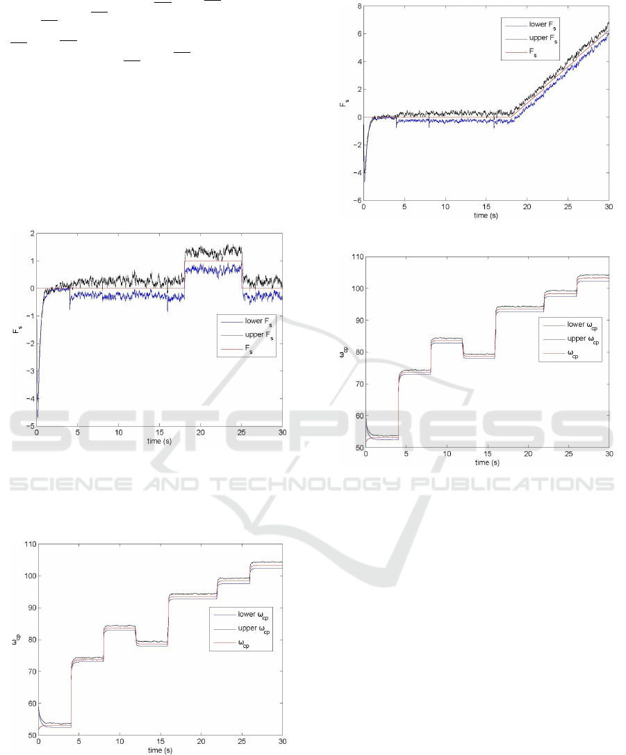
Case 1.- Abrupt Fault.

An abrupt fault occurs from 18 to 25 sec affecting the

speed sensor. Figure 6 presents the interval estimation

that for this case the observer (28) can estimate.

Figure 6: Estimation of f

The state estimation of the TS system with the

fault affecting the speed sensor is shown in the Fig-

ure 7.

Figure 7: Estimation of ω

Case 2.- Incipient Fault.

Figure 8 illustrates the interval fault estimation when

the incipient fault is applied in the output sensor. The

state estimation is presented in the Figure 9.

Figure 8: Estimation of f

Figure 9: Estimation of ω

5 CONCLUSION

In this paper, an approach for estimating faults using

the TS interval observer is proposed. Faults are con-

sidered as an additional state in the observer model.

The proposed method allows to obtain the estimation

of faults and state simultaneous. In case that observ-

ability conditions are satisﬁed FDI is not required.

Otherwise, it should be used combined with a bank

of observers dedicated to a subset of faults. The pro-

posed approach have been satisfactorily tested on the

compressor of fuel cell system in several scenarios in-

cluding abrupt and incipient faults. As a future work,

the proposed scheme will extended to process faults

and to the case of unmeasured premise variables.

ACKNOWLEDGMENTS

This work has been partially funded by the Spanish

Government (MINECO) through the project ECO-

Fault Estimation using a Takagi-Sugeno Interval Observer: Application to a PEM Fuel Cell

619

CIS (ref. DPI2013- 48243-C2-1-R), by MINECO

and FEDER through the project HARCRICS (ref.

DPI2014-58104-R).

REFERENCES

Aouaouda, S., Boukhnifer, M., and Bouhali, O. (2014).

Sensor fault observer design for uncertain Takagi-

Sugeno Systems. In In 2014 IEEE 23rd International

Symposium on Industrial Electronics (ISIE), pages

236–241.

Blanke, M., Kinnaert, M., Lunze, J., and Staroswiecki,

M. (2006). Diagnosis and Fault-Tolerant Control.

Springer-Verlag.

Brune, B. and F, M. (2001). Detecting leaks in pressurised

pipes by means of transients. Journal of hydraulic

research, 39(5):539–547.

Chilali, M. and Gahinet, P. (1996). H

∞

design with pole

placement constraints: an LMI approach. Birches J,

41(3):358–367.

Eﬁmov, D., Rassi, T., and Zolghadri, A. (2013a). Control

of nonlinear and lpv systems: Interval observer-based

framework. In IEEE Transactions on Automatic Con-

trol, volume 58, pages 773–778.

Eﬁmov, D. V., Rassi, T., Perruquetti, W., and Zolghadri, A.

(2013b). Estimation and control of discrete-time lpv

systems using interval observers. In Proceedings of

the IEEE 52nd Annual Conference on Decision and

Control (CDC), pages 5036–5041.

Guerra, T. M., Estrada-Manzo, V., and Lendek, Z. (2015).

Observer design for Takagi-Sugeno descriptor mod-

els: An LMI approach. Automatica, 52:154–159.

Ho, W. H., Chen, S. H., and Chou, J. H. (2013). Observabil-

ity roburobust of uncertain fuzzy-model-based control

systems. International Journal of Innovative Comput-

ing, Information and Control, 9(2):805–819.

Hwang, I., Kim, S., Kim, Y., and Seah, C. E. (2010). A

survey of fault detection, isolation, and reconﬁgura-

tion methods. IEEE Transactions on Control Systems

Technology, 18(3):636–653.

Ichalal, D., Marx, B., Ragot, J., and Maquin, D. (2010).

Brief paper: state estimation of Takagi-Sugeno sys-

tems with unmeasurable premise variables. IET Con-

trol Theory & Applications, 4(5):897–908.

ofberg, J. (2004). YALMIP : A toolbox for modeling and

optimization in MATLAB. In Computer Aided Con-

trol Systems Design, 2004 IEEE International Sympo-

sium on.

Mahmoud, H., Jiang, J., and Zhang, Y. (2003). Active fault

tolerant control systems. Berlin:Springer-Verlag.

Noura, H., Theilliol, D., and J, C. (2009). Fault-tolerant

control systems: design and practical applications.

Berlin:Springer-Verlag.

Puig, V. (2010). Fault diagnosis and fault tolerant control

using set-membership approaches: Application to real

case studies. International Journal of Applied Mathe-

matics and Computer Science, 20(4):619–635.

Pukrushpan, J. T., Peng, H., and Stefanopoulou, A. G.

(2004). Control-oriented modeling and analysis for

automotive fuel cell systems. Journal of dynamic sys-

tems, measurement, and control, 126(1):14–25.

Rassi, T., Videau, G., and Zolghadri, A. (2010). Inter-

val observer design for consistency checks of nonlin-

ear continuous-time systems. Automatica, 46(3):518–

527.

Rotondo, D., Fernandez-Canti, R. M., Tornil-Sin, S., Blesa,

J., and Puig, V. (2016). Robust fault diagnosis of

proton exchange membrane fuel cells using a Takagi-

Sugeno interval observer approach. International

Journal of Hydrogen Energy, 41(4):2875–2886.

Samy, L., Postlethwaite, L., and Gu, D. W. (2011). Survey

and application of sensor fault detection and isolation

schemes. Control Engineering Practice, 19(7):658–

874.

Takagi, T. and Sugeno, M. (1985). Fuzzy identiﬁcation of

systems and its application to modeling and control.

IEEE Transactions on Systems, Man, and Cybernet-

ics, SMC-15:116–132.

Wee, J. H. (2007). Applications of proton exchange mem-

brane fuel cell systems. Renewable and Sustainable

Energy Reviews, 11(8):1720–1738.

Witczak, M. (2007). Modelling and Estimation Strategies

for Fault Diagnosis of Non-linear Systems: From An-

alytical to Soft Computing Approaches. Lecture Notes

in Control and Computer Science.

Witczak, M. (2014). Fault diagnosis and fault-tolerant con-

trol strategies for non-linear Systems. Springer.

Zhang, K., B, J., and Shi, P. (2009). A new approach

to observer-based fault-tolerant controller design for

Takagi-Sugeno fuzzy systems with state delay. Cir-

cuits, Systems and Signal Processing, 28(5):679697.

Zhang, Y. and Jiang, J. (2008). Bibliographical review on

reconﬁgurable fault-tolerant control systems. Annual

Reviews in Control, 32(2):229–252.

ICINCO 2017 - 14th International Conference on Informatics in Control, Automation and Robotics

620