
Inverse Response Systems Identification using Genetic Programming
Carmen Alicia Carabal
´
ı
1,2
, Luis Titua
˜
na
1
, Jose Aguilar
1,2
, Oscar Camacho
1,2
and Danilo Chavez
1
1
Escuela Polit
´
ecnica Nacional, Quito, Ecuador
2
Universidad de los Andes, M
´
erida, Venezuela
Keywords:
Genetic Programming, Inverse Response, System Identification.
Abstract:
In this paper, we apply genetic programming as a tool for identifying an inverse response system. In previous
works, the genetic programming has been used in the context of identification problems, where the goal is to
obtain the descriptions of a given system. Identification problems have been studied much from control theory,
due to their practical application in industry. In some cases, a description of a system in terms of mathematical
equations is not possible, for these cases are necessary new heuristic approaches like the genetic programming.
Here, we like to test the quality of the genetic programming to identify inverse response systems, which are
systems where the initial response is in a direction opposite to the final outcome. The tool used to develop the
model of identification is GPTIPS V2, we use our approach in two cases: in the first one, the equation that
describes inverse response system is determined; and in the second case, the transfer function of the system in
the frequency domain is found.
1 INTRODUCTION
In chemistry, robotics, mechanics, etc, there are a lot
of systems with different inputs and outputs. Usually,
there is a need for knowing the mathematical model
that describes the behavior of these systems, for un-
derstanding their working principles and analyze how
to control them. However, there are cases where there
is not information about the dynamical behavior of
the system, therefore is necessary to identify it using
the available data, as for example, the values of inputs
of the process and their correspondent outputs, useful
information for obtaining an approximate mathemat-
ical model of the process. In general, the purpose of
system identification is to obtain its description. Nor-
mally, this descriptions made in terms of mathemat-
ical equations, but when it is used data for this task,
heuristic techniques can be used.
In general, there exist a group of different tech-
niques used to determinate the model of a system
(Chinarro, 2014), the classical ones based on the anal-
ysis of the response of the system to the step sig-
nal (Kopka, 2014), others which use optimization for
minimizing an error (Lyzell, 2009), the ones based on
geometrical calculations, and those based on artificial
intelligence for system identification (Samy et al., ),
(Mishra and Giri, 2014). When the systems have a
nonlinear behavior, it is important to consider them
as a particular case, as a consequence, new exclusive
methods must be proposed for their identification.
Particularly, in this case we propose to use ge-
netic programming to solve the problem of nonlinear
systems identification, and in specific, an inverse re-
sponse system that is very complex to model math-
ematically. Genetic programming has revolutionized
the classic approach for problem solving using com-
puters. It is based on the evolutionary process of the
species to solve any class of problem, by always fol-
lowing the same algorithm. Here, we propose two dif-
ferent approaches for system identification based on
genetic programming, and we will use the GTIPS V2
tool developed by Dominic Searson (Searson, 2015).
In the first one, we search the equation that describes
the system; and in the second one, we search the
transfer function in the frequency domain.
The rest of the paper will be organized as follows,
the section 2 will present the principles related with
genetic programming, inverse response systems and
system identification methods, the third section will
explain the proposed approach for system identifica-
tion, in the fourth section are shown the obtained re-
sults, and finally, section five contains the final dis-
cussion and the conclusions related with the obtained
results.
238
Carabalí, C., Tituaña, L., Aguilar, J., Camacho, O. and Chavez, D.
Inverse Response Systems Identification using Genetic Programming.
DOI: 10.5220/0006421602380245
In Proceedings of the 14th International Conference on Informatics in Control, Automation and Robotics (ICINCO 2017) - Volume 1, pages 238-245
ISBN: 978-989-758-263-9
Copyright © 2017 by SCITEPRESS – Science and Technology Publications, Lda. All rights reserved
2 CONTEXT
In this document we present an alternative method for
the identification of systems with inverse response us-
ing genetic programming. Then, there is a brief de-
scription of Inverse Response Systems, System Iden-
tification Techniques and Genetic Programming.
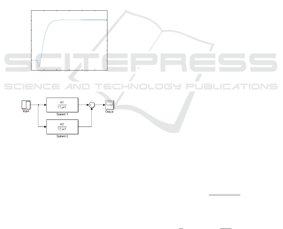
2.1 Inverse Response Systems
Inverse response systems are systems with a particu-
lar characteristic, at the beginning of the process, the
output instead of get closer to the desired set point, it
tends to go in the opposite direction, as can be seen
in Figure 1. The reason why this happens respond to
the nature of the system; ideally, it can be modeled
as the difference of two first order systems, as it is
shown in Figure 2.
0 2 4 6 8 10 12
Time
1.09
1.1
1.11
1.12
1.13
1.14
1.15
Output
Inverse Response
Figure 1: Typical output of an inverse response system.
Figure 2: Inverse response system modeled as the difference
between two first order systems.
For obtaining an inverse response, K
1
> K
2
and
the reaction of the system 1 has to be slower than the
reaction of system 2.
Inverse response is typical when two effects are
occurring at the same time, but with different dynam-
ics and directions. Thus, the system has two transfer
functions coupled in parallel, so the individual out-
puts can be added to obtain the overall response.
These systems are difficult to control , because
they can easily have stability problems in the con-
trol loop (Hongdong et al., 2005), and have always
been a challenge because the efficiency of the systems
depends on the way how they are controlled (Pant,
2012). Additionally, it results complicated to obtain
the model of the system, from their inputs and out-
puts. Examples of these kind of systems are: a drum
boiler, a stirred reactor, an exothermic tubular reactor,
among others.
2.2 Non Linear Systems Identification
Since 70s a large number of methods for system
identification have been developed, these methods
can be organized in 7 groups: linearization methods,
time and frequency-domain methods, modal methods,
time-frequency analysis methods, black-box model-
ing and structural model. Most of the methods use
least squares or maximum likelihood estimation, but
most of the time, both techniques, are not able to find
the global maximum when the parameters are non lin-
ear.
A nonlinear system means that its output to a
weighted sum of input signals is not the weighted sum
of responses to each of the input signals. Classically,
the identification of these systems is very hard, and
approximative methods are required, in order to ob-
tain models close to their real behavior.
Most common methods for non linear systems
identification, and more specific inverse response, are
based on graphical approaches, where the data curve
is used as starting point for the deduction of the struc-
ture of the model. Then, from some points chosen in
the curve, parameters can be determined in that struc-
ture of the model. This method is used in the works
of (Esakkiappan and Thyagarajan, 2012), (Luyben,
2003), (Balaguer et al., 2011).
In (Luyben, 2003) is used the data curve with a
known structure, which is shown in Equation 1. For
getting the values of the constants: K
P
, τ
1
and τ
2
,
the author determines the function that represents the
curve in the time domain, which is shown in the Equa-
tion 2, and its derivative is Equation 3. Later on, in
this work he chooses two points; the one where the
response of the system reach its minimum value (t
1
)
and the point where the value of the function is 0 (t
2
).
With this information, they solve Equations 4 to 6.
This procedure determinates the constants and as a
consequence, the model of the system.
G(s) =
K
p
(−τ
1
s+1)e
−Ds
(τ
2
s+1)s
(1)
y(t) = ∆uK
p
t − τ
1
− τ
2
+ (τ
1
+ τ
2
)e
−t/τ
2
(2)
dy
dt
= ∆uK
p
h
1 −
τ
1
+τ
2
τ
2
e
−t/τ
2
i
(3)
A t=t
1
:
y(t)
min
= ∆uK
p
t − τ
1
− τ
2
+ (τ
1
+ τ
2
)e
−t/τ
2
(4)
Inverse Response Systems Identification using Genetic Programming
239

dy
dt
= 0 = ∆uK
p
h
1 −
τ
1
+τ
2
τ
2
e
−t/τ
2
i
(5)
A t=t
2
:
y(t) = 0 = ∆uK
p
t − τ
1
− τ
2
+ (τ
1
+ τ
2
)e
−t/τ
2
(6)
Other authors propose the use of a Relay Feedback
test, see for more detail (Esakkiappan and Thyagara-
jan, 2012). In this case, the authors apply a chang-
ing relay as input signal, obtained as output the signal
shown in Figure 3. From the output curve some points
as: t
max
y
max
, t
z
and y
z
are chosen in order to calcu-
late the constant K
p
, τ
1
, and τ
2
of the model shown
in Equation 7. The constant D is obtained directly
for the output curve, determining the delay between a
zero crossing point at the moment when the slope of
the curve changes drastically.
Figure 3: Relay response of the process taken from (Esakki-
appan and Thyagarajan, 2012) .
G(s) =
K
p
(−τ
1
s+1)e
−Ds
(τ
2
s+1)s
(7)
Finally, the system identification method of Bal-
aguer (Balaguer et al., 2011) has become very pop-
ular. He proposes a method for the identification of
second order inverse response systems. It consists
in the selection of three points on the output curve:
(t
x
,y
x
), (t
y
,y
y
) and (t
p
,y
p
) being the last one the neg-
ative peak. The information of the points is used in the
Equations 8, 9, 10 and 11. Finally, the obtained values
are incorporated in the Equation 12, which represent
the model of the system.
K =
∆y
∆u
(8)
T 1 =
t
y
−t
x
ln
y
y%
−1
y
x%
−1
(9)
b = 1 −
1−t
p%
e
t
0
p
(10)
a =
t
0
z
−
(
m
1z
+m
3z
b+m
5z
b
2
)
(
m
2z
+m
4z
b+m
6z
b
2
)
(11)
G(s) =
K
1
T
1
S+1
−
K
2
T
2
S+1
e
−hs
(12)
Where K is the gain of the system, y and u, the
input and output, respectively.
The Equations 13, 14, 15 and 16 help to obtain the
parameters of the Equation 5.
K
1
= K
1−b
1−a
(13)
K
2
= K
a−b
1−a
(14)
K
=
K
1
− K
2
(15)
T
3
=
K
1
T
2
−K
2
T
1
K
1
−K
2
(16)
The three previous methods, are representative of
the approaches that have been commonly used for
inverse response system identification, all them are
graphical methods that need the output curve for char-
acterizing the system. Here, we propose a different
approach using artificial intelligence techniques for
system identification.
2.3 Genetic Programming
Genetic programming is an artificial intelligence tech-
nique used for symbolic optimization based on the
evolutionary process of the species (Madar et al.,
2004). It was developed by John Koza (Koza, 1998),
and has as principle the combination of trees used to
represent symbolic expressions.
Genetic programming is a technique where the au-
tomatic learning is involved, and it is based on the
natural evolution. Specifically, it consist, in the ran-
dom generation of a certain number of genes, which
are combined in order to create a new population of
genes. The combination operation is repeated con-
stantly, and in each iteration there is a mutation of
the genes. The iteration stops when the best model is
found or certain stop condition is met.
In our case, the genetic programming evolves a
set of functions capable of relate the variables of the
system, in order to describe its output. Genetic pro-
gramming is capable of building trees that describe
the system, using a large set of operators (e.g. arith-
metics, logics, trigonometrics, exponentiation, loga-
rithmic functions, etc.).
Genetic programing has a number of basics steps
for its execution, which are presented in (Poli et al.,
2008):
• Creation of the initial population of individuals in
a random way.
• Repeat.
– Evaluation of each individual using the fitness.
– Select of one or two individuals to participate
in the reproduction phase.
ICINCO 2017 - 14th International Conference on Informatics in Control, Automation and Robotics
240

– Reproduction of the individuals by applying ge-
netic operators.
• Until an acceptable solution is found or a stopping
condition is met.
• Return the best individual.
Particularly, the fitness function determine the
quality of the individuals (equations) to follows the
behavior (description) of the system.
3 APPROACH OF SYSTEM
IDENTIFICATION BASED ON
GENETIC PROGRAMMING
Based on section 2.2, it can be deduced that for sys-
tem identification the common approach is to assume
an initial structure, then, to find the value of the con-
stants in it using the curve of the output data. How-
ever, there are cases where there is not previous in-
formation about the type of the system, and therefore,
it is complicated to know the structure and order of
it. As an alternative, we propose the use of the ar-
tificial intelligence in order to determine the model
of the system, where there is not need of previous
information about its characteristics. The use of the
artificial intelligence for system identification is not
new, it has been applied before by different research
groups (Chen et al., 1990), (Cerrada and Aguilar,
2001), (Patelli, 2011), (Madar et al., 2004), (Samy
et al., ), among others.
The decision of using genetic programing is based
in the fact that this technique does not provide unique
responses, instead it generates a population of solu-
tions which can fit the model of the system. This fea-
ture gives to the researcher the possibility of choos-
ing, a determined structure, according to the level of
complexity or the precision of the model required by
the context of the application.
In this work, we propose the implementation of
two different methods for the system identification.
The first one, uses information about the inputs and
the outputs of the system, which are used to establish
the relationships between them in the time domain,
which can be associated to a non linear system.
The second proposed method helps to determine the
relationship between inputs and outputs, through
the transfer function of the system in the frequency
domain, which is necessarily associated to a linear
system.
The Genetic Programming tool used is the GP-
TIPS V2 Toolbox for MATLAB, developed by Do-
minic Searson. It carries out a multi gene symbolic
regression, with input-output data. Each symbolic
model obtained (a member of the GP population) is a
weighted equation that is a combination of the inputs
of the system (Searson, 2015), plus a bias term. The
weights are calculated with an ordinary least squares
technique.
The tool uses an elitist selection mode, where the
best individuals of the population are chosen to be-
come the parents of new ones, or to be the final mod-
els, depending of the least Root Mean Square Er-
ror (RMSE). However, this criteria presents a poten-
tial disadvantage, the models obtained might be too
complex. In other words, the mathematical functions
within the models could be very intricate, i.e. mul-
tiple nested functions, which represents a difficulty
when giving a physical interpretation of the system,
and subsequently, greater difficulty in the design of a
controller. To solve this, the depth of the trees created
by the GP and the number of genes (trees) have to be
limited and the chosen mathematical functions must
define simple models structures.
One of the most critical parts of the identification
is the acquisition of the data from the plant, which will
be used to train and test the models. Since we want
information of its transient response (due to sudden
changes in the input) and its steady state behavior, the
number of data taken must be chosen appropriately to
reflect these events. If the proportion of data obtained
from the transient part is similar or less than the por-
tion of the steady state data, then the obtained model
will present a steady-state error, which is undesirable.
This happens because the program chooses the indi-
viduals that produce the least RMSE, thus, those in-
dividuals with their transient responses more similar
to the real plant are chosen (since most of the data
comes from that time). To avoid this, the chosen pro-
portion of data was 0.1, that is, 1 transient data for
every 10 of the steady state. The final population of
individuals will be the union of the best individuals
after 10 different runs. The criterion of termination of
the program will be when one of the models reaches
an RMSE of 0.01.
3.1 Method 1: Obtaining the Equation
that Describes the System Behavior
For determining the equation that describes the rela-
tionship between the inputs and the output of the sys-
tem, the next steps were performed:
1. Get the data from of the system, including all the
inputs and the outputs of the system.
2. Use GP to determine a set of individuals that de-
scribe accurately the relationship between the in-
Inverse Response Systems Identification using Genetic Programming
241
puts and the output of the system. The parameters
used are displayed in Table 1.
3. Choose the best individuals, which are the indi-
viduals with RMSE close to 1 and a small level
of complexity, using the popbrowser function of-
fered by GPTIPS V2.
4. Repeat the steps 2 and 3, for inputs contaminated
with certain amount of noise, simulating noise
that can be present in the data acquisition process.
5. Repeat the steps 2 and 3 for different inputs.
6. Compare the results from numerals 3, 4 and 5, and
determinate a model to describe the system.
Table 1: Parameters used for GP, for the first approach.
Parameter Value
Population size 100
Generations 100
Number of Runs 1
Elite Fraction 0.15
Tournament size 6
Max tree depth 2
Max genes 3
Functions set +,−,∗,/, exp, square
3.2 Method 2: Obtaining the Transfer
Function of the System in ihe
Frequency Domain
The method for obtaining the transfer function that
describes the behavior of the system in the frequency
domain is defined by the next steps:
1. Use GP with the parameters show in Table 2, to
get a set of functions that describe the output of
the system in function of the time.
2. Select a function of the set of functions, using the
popbrowser function of the tool.
3. Transform the output of the system, Y (s), to the
frequency domain using the Laplace transform.
4. Transform the input of the system, X(s), to the
frequency domain.
5. Divide the output of the system Y (s) to the input
of the system X(s), to obtain the transfer function
in the frequency domain.
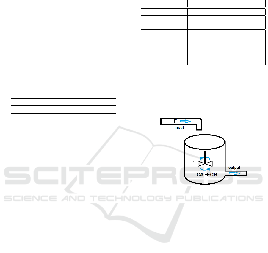
4 EXPERIMENTS
For testing the methods developed, the model of a
known inverse response system was used. It is the Van
Table 2: Parameters used for GP, for the second approach.
Parameter Value
Population size 1000
Generations 1000
Number of Runs 10
Elite Fraction 0.15
Tournament size 6
Max tree depth 2
Max genes 4
Functions set +,−,∗,/, exp, square,sin,cos
de Vusse reactor, represented in the Figure 4, where
the Flux, (F) and the concentration A, (CA), are the
input variables, and the concentration B, (CB) is the
output. CA depends of F, and CB depends of a chem-
ical reaction in which CA is involved. Equations 17
and 18 describe the dynamics of the system.
Figure 4: Van de Vusse Reactor scheme.
dCA(t)
dt
=
F(t)
V
[CA
i
−CA(t)] − k
1
CA(t) − k
3
CA
2
(t) (17)
dCB(t)
dt
= −
F
V
CB(t) + k
1
CA(t) − k
2
CB(t) (18)
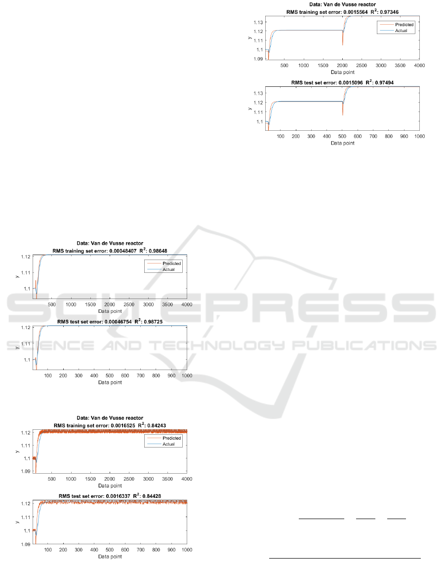
4.1 Relationship between the Inputs
and the Output of the System
The data used was obtained from a model imple-
mented in Simulink from MATLAB based on Equa-
tions 17 and 18. Three experiments were perfomed, in
the first one the flux followed an step function with an
initial value equal to 380 and a final value 439, with
the step one second after of the beginning the pro-
cess. In the second experiment the same inputs were
used, however, there was some noise added to them,
simulating the noise existing when data is being ac-
quired. Finally, the third experiment consisted in a
flux changing two times as step functions, from 380
to 410 and from 410 to 439.
After performing the genetic programming algo-
rithm using GPTIPS V2 for each one of the experi-
ments, a group of 100 different functions was gener-
ICINCO 2017 - 14th International Conference on Informatics in Control, Automation and Robotics
242
ated. In Table 3 are shown the best individuals ob-
tained in each experiment, considering the complex-
ity and R
2
, which is a constant from 0 to 1, found us-
ing statistical methods that provide information about
how good an obtained curve fits to a given one.
For the first experiment, the individual 75 has a
very good performance, but it is very complex. In the
third experiment are obtained good individuals, and
some of them are not complexes (e.g., the individuals
87, 51). These individuals are a good alternative to
chose.
After analyzing the resultant functions, it is car-
ried out the definition of an standard model to de-
scribe the system obtained, which is modeled by the
function in the Equation 19.
CB = c
1
CA − c
2
F +0.3 (19)
Where c
1
and c
2
are constants, to determine a stan-
dard model that fits different functions with similar
features
Figure 5: Response to the Flux as a Step input.
Figure 6: Response to the Flux as a step input and simula-
tion of noise during the data collection.
Figure 7: Response to the Flux as a step input varying twice
along time.
4.2 Transfer Function in the Frequency
Domain
The data used was obtained from a model im-
plemented in Simulink from MATLAB, based on
Equations 17 and 18. The input was a flux signal
following a Step function with amplitude equal to
430.
For obtaining the transfer function in the fre-
quency domain, the steps in 3.2 were followed. After
performing the genetic programming, the Equation 20
was obtained. The parameters used are shown in Ta-
ble 2. The duration of the calculation was about 0.95
minutes, as there was just one input variable: ’time’.
The population chosen was of 1000 individuals, and
the number of generation was 1000, the number of
runs performed was 10.
CB = 1.14 − 0.0471e
−t
− 0.0495te
−t
− 2.08x10
−5
t
(20)
The obtained output in the time domain was trans-
formed to the frequency domain using Laplace. The
resultant function is the Equation 21. It was divided
by the input transformed to the frequency domain, ob-
taining the transfer function shown in Equation 22.
Y (s) =
0.1s−2.08x10
−5
s
2
−
0.0495
(s+1)
2
−
0.0471
s+1
(21)
H(s) =
2.54x10⁻³s
3
+5.079x10
−3
s
2
+2.66x10
−
3s−4.89x10
−
8
s(s+1)
2
(22)
The comparison between the actual output and the
obtained output with the new identified transfer func-
tion is shown in Figure 8. The average error R
2
from
the comparison was 0.94256.
Inverse Response Systems Identification using Genetic Programming
243

Table 3: Best individuals for each experiment, considering error and complexity.
Experiment Resultant Function R
2
Individual
1 CB = 0.0002F − 13.56CA + 0.70e
CA
+ 27.55 0.986 75
1 CB = 0.019e
CA
− 6.9x10
−4
F + 1 0.908 54
1 CB = 0.37CA − 7x10
−4
F + 0.29 0.904 9
2 CB = 0.0158e
CA
− 0.0004584F +0.9801 0.84243 75
2 CB = 0.32CA − 4.8x10
−4
F + 0.36 0.84182 11
3 CB =
−
(
1.649CA−0.0374F+0.013CAF+0.34CA
3
)
CA
0.97346 69
3 CB = 0.062CA
2
− 7x10
−4
F + 0.85 0.97002 87
3 CB = 0.36CA − 6.9x10
−4
F + 0.3 0.96985 51
500 1000 1500 2000 2500 3000 3500 4000
Data point
1.1
1.12
1.14
y
Data: Van de Vusse reactor
RMS training set error: 0.0020504 R
2
: 0.94256
Predicted
Actual
100 200 300 400 500 600 700 800 900 1000
Data point
1.1
1.12
1.14
y
RMS test set error: 0.0020471 R
2
: 0.94222
Figure 8: Comparison of two responses, the Predicted gen-
erated by our individuals and the Actual, the original one.
5 CONCLUSIONS
In this paper we have proposed an alternative to the
most traditional methods for system identification us-
ing genetic programming for determining the dynam-
ics of the system. This technique is based on a ’nat-
ural selection’ of the individuals, in order to allow
the best fitness functions to survive. The advantages
of the use of this technique are the fact that there is
not need to know the order of the system and a pre-
established structure, and that it provides population
of solutions, from which the most suitable can be se-
lected according to certain criteria of selection.
We propose two methods, in order to define a good
model to represent the relationship between the input
data and the output data. In the first case we have de-
fined three different experiments to identify a model
that is presented in the equation 19, which can be con-
sidered as standard for an specific process, the Van de
Vusse Reactor. Future work will imply the use of Ge-
netic Programming for identifying standard models
for other processes. Also, it is necessary the develop-
ment of new methods for calculating the constants to
adjust the standard models found for different systems
with similar features. For example, for the Equation
19 for determining constants c
1
and c
2
.
The second method developed uses the genetic
programming to identify the expression that relates
the output and the input in the frequency domain. In
this case, there was a need of a bigger amount of genes
and multiple runs. There was a compromise between
complexity and a more accurate model with R
2
closer
to one, therefore, the selection of the individual from
the population to use was made carefully.
In the case of the second method, a better func-
tion, could be obtained if trigonometric functions are
added to the genetic programming. Additionally, fu-
ture works, will imply the consideration of the weight
of each one of the genes of the selected individuals.
Genes with small weights will be dismissed, decreas-
ing the complexity of the transfer function obtained.
One of the advantages of the proposed methods
is that the technique used, Genetic Programming, is
not sensitive to the variations in the data. Therefore,
small interferences as noise, for example, do not af-
fect the obtained model drastically, as is shown in the
Figure 6 for the second experiment. In the other hand,
the models found using the technique, provide a rela-
tionship between inputs and outputs, therefore, they
are highly sensitive, making possible that any small
change in the input, could cause an effect in the out-
put. Finally, the nature of the Genetic Programming
makes our proposed approach immune to the effects
of non linearities because it just looks for the better
fit.
In general it can be said that the proposed methods
are capable of providing accurate and compact mod-
els. Here, were presented two approaches to solve the
identification problem, one in which were considered
only the relationships between the inputs and the out-
put in the time domain, and another in which a trans-
fer function of the system was determined in the fre-
quency domain.
ICINCO 2017 - 14th International Conference on Informatics in Control, Automation and Robotics
244

ACKNOWLEDGEMENTS
Dr Aguilar and Dr Camacho have been partially sup-
ported by the Prometeo Project of the Ministry of
Higher Education, Science, Technology and Innova-
tion of the Republic of Ecuador.
REFERENCES
Balaguer, P., Alfaro, V., and Arrieta, O. (2011). Second or-
der inverse response process identification from tran-
sient step response. ISA Transactions, 50(2):231–238.
Cerrada, M. and Aguilar, J. (2001). Genetic Programming-
Based Approach for System Identification. Advances
in Fuzzy Systems and Evolutionary Computation, Ar-
tificial Intelligence, pages 329–334.
Chen, S., Billings, S. A., and Grant, P. M. (1990). Interna-
tional Journal of Control. (769892610).
Chinarro, D. (2014). System Identification Techniques.
Esakkiappan, C. and Thyagarajan, T. (2012). Identification
of Inverse Response Process with Time Delay Using
Relay Feedback Test. Int. J. Comput. Appl. Technol.,
44(4):269–275.
Hongdong, Z., Guanghui, Z., and Huihe, S. (2005). Control
of the Process with Inverse Response and Dead-time
based on Disturbance Observer. pages 4826–4831.
Kopka, R. (2014). A Simple Method for Estimation of Pa-
rameters in First order Systems. Journal of Physics:
Conference Series, 570.
Koza, J. (1998). Genetic Programming : On the Program-
ming of Computers By Means of Natural Selection
Complex Adaptive Systems.
Luyben, W. (2003). Identification of integrating processes
with deadtime and inverse response. Industrial and
Engineering Chemistry Research, 46(42):3030–3035.
Lyzell, C. (2009). Initialization Methods for System Identi-
fication. Number 1426.
Madar, J., Abonyi, J., and Szeifert, F. (2004). Genetic Pro-
gramming for System Identification.
Mishra, P. and Giri, A. (2014). Review of system identifica-
tion using neural network techniques 1 1,2. (7):13–16.
Pant, B. (2012). Taming inverse response. (July).
Patelli, A. (2011). Genetic Programming Techniques for
Nonlinear Systems Identification. Ed. Politehnium.
Poli, R., Langdon, W. B., Sciences, M., Mcphee, N. F., and
Koza, J. R. (2008). A Field Guide to Genetic Pro-
gramming. Number March.
Samy, W., Elshamy, M., and Power, E. Using Artificial
Intelligence Models in System Identification. (May
2007).
Searson, D. P. (2015). GPTIPS 2: an open-source software
platform for symbolic data mining. (c).
Inverse Response Systems Identification using Genetic Programming
245
