Mixed Fluid and Rigid Body Simulations

An Object Oriented Component Library based on the Physolator Framework

Waldemar Rose and Dirk Eisenbiegler

University of Furtwangen, Furtwangen, Germany

Keywords: Particle Modelling, Fluid Simulation, Rigid Body Simulation, Physolator, Java Framework, Object Oriented

Modelling.

Abstract: This paper presents an approach towards implementing physical simulations, where the physical system

consists of both fluids and movable rigid bodies. The approach is based on Physolator. Physolator is an

object oriented Java based framework for physical simulation. This paper introduces a library of Java

classes that are designed for building such simulations. The classes are designed to be used inside the

Physolator framework.

1 INTRODUCTION

Physical simulation is used in different domains and

there are various software tools tailored to the

specific needs of such domains. Fluid simulations

and rigid body simulations are such domains.

Fluid simulations describe the flow of gases and

liquids. A fluid simulation describes the actual

location of the fluids for each point in time, the

forces applied to the fluids and physical fields for

the flow velocity and pressure. Particle models are

frequently used for computer based physical

simulations (Greenspan, 1997, 1985, 2004,

Nijmeijer, 1992, Korlie, 1997, 1999, Pozrikidis,

2017). Particle simulations are challenging. It takes a

big number of particles to achieve a reasonable

accuracy. Therefore, such simulations usually

require big amounts of computing time.

Programmers have to spend a lot of time for

optimizations in order to achieve a reasonable

simulation accuracy within a limited computation

time.

Rigid body mechanics is about physical bodies,

that are not deformable. During the simulations, the

rigid bodies move, the shape however remains

unchanged. Different kinds of forces can apply to a

rigid body during simulation: gravity, magnetic

forces, sliding friction, static friction, rolling

friction, etc.. These forces accelerate rigid bodies

and change their translational and rotational

velocity. Furthermore, there are collisions between

rigid bodies. Collisions abruptly change the

translational and rotational velocity of the bodies

involved. Rigid body simulations are frequently used

in computer games and animated films. Game

engines usually contain a component named

“physics engine”. This kind of physics engine is

usually limited to rigid body physics. From a

computational point of view, rigid body simulations

are far less challenging than fluid simulations.

Physics engines inside computer games are designed

for real time execution. For a limited amount of

components, they succeed computing frames within

milliseconds. In a computer game, the accuracy of

the physical computation has to be reasonable in a

sense that the user of the computer game should get

the impression, that the virtual world of the

computer game behaves just like the real world.

Simulations inside computer games need not

necessarily produce results, that are precise in a

scientific sense.

This paper is about physical systems consisting

of both fluids and rigid bodies. Concepts from both

worlds, fluid simulation and rigid body simulation,

are to be applied. The next section describes how

such physical systems look like and gives an

example. The following section explains the concept

used to create models for such physical systems and

it explains, how to run such simulations. Finally,

there will be a section with algorithmic

considerations. Whenever you deal with particle

simulations, computing time matters. The final

section describes the algorithms and the concurrency

Rose, W. and Eisenbiegler, D.

Mixed Fluid and Rigid Body Simulations - An Object Oriented Component Library based on the Physolator Framework.

DOI: 10.5220/0006402600360044

In Proceedings of the 7th International Conference on Simulation and Modeling Methodologies, Technologies and Applications (SIMULTECH 2017), pages 36-44

ISBN: 978-989-758-265-3

concepts used inside the library in order to achieve a

good performance.

2 MIXED FLUID AND RIGID

BODY SYSTEMS

This section describes, how physical systems with

fluids and rigid bodies look like. Using an example,

it is explained, what kind of components are used to

build up such systems and which physical effects

have to be considered.

Figure 1 shows a sequence of snapshots from a

physical simulation with water and rigid bodies. In

picture (I) you can see a basin filled with water. A

water drop is about to fall into the basin. The floor

of the basin and the wall on the left hand side are

fixed. On the right hand side of the basin, there is a

rectangular solid block. The block lies on the basin

floor. In the beginning, the block does not move.

Figure 1: Simulation with water and rigid bodies.

The water inside the basin applies a force

towards the block pushing the block rightwards.

Static friction, however, hinders the block from

moving. The static friction force is a counterforce to

the force from the water with the same absolute

value, but opposite direction. Static friction applies

as long as the block is not in motion and as long as

the force applied to the block does not exceed a

certain maximum. The maximal static friction force

is a constant. It depends on the force the block

applies to the floor of the basin and a static friction

coefficient. In the beginning, the absolute value of

the force from the water is smaller than the maximal

friction force.

As soon as the water drop falls inside the basin,

the force applied to the block increases. At a certain

point in time (II), this force exceeds the maximal

static friction force and the block starts moving

rightwards. At this point in time, static friction is

replaced by sliding friction. The sliding friction is

smaller than the static friction. Sliding friction

applies as long as the block is in motion. As soon as

the block moves to the right, also the water starts

moving rightwards (III). Since the water moves

rightwards, the water level inside the basin is

decreased. As a consequence, the force from the

water applied to the block lessens. As soon as this

force is smaller than the sliding friction, the total

force applied to the block is directed to the left. The

block is slowing down and finally stops (IV). As

soon as the block stops, sliding friction is replaced

by static friction and the block remains in this final

position.

Different kinds of physical effects have to be

considered when performing this simulation: forces

between the water particles, internal friction, forces

between the liquid and the rigid bodies, static

friction, sliding friction. Some of these effects are

related to fluid physics and some to solid body

physics.

Basically, the relationship between the physical

variables involved can be described via differential

equations. However, also points of discontinuity

have to be considered. At the point in time, when the

block starts moving, the static friction abruptly

vanishes and is replaced by sliding friction. At the

point in time, when the block stops moving, it is the

other way round: sliding friction is replaced by static

friction. Physical simulations are an appropriate

means for answering question like these: When will

the block start moving? How far will it move? When

will it stop moving?

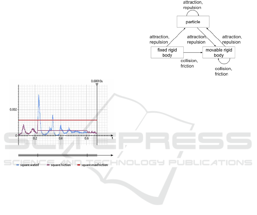
Figure 2 shows a function plot with some of the

physical variables involved in this simulation. This

diagram shows the forces applied to the block. The

upper horizontal line represents a constant: the

maximal static friction. In the beginning, there are

two forces with the same absolute value: the force,

that the water applies to the block and the static

friction force. The value of this force is continuously

changing due to the movement of the water. As soon

as the force from the water reaches the maximal

static friction force, the block starts moving. As long

as the block is moving, there is still the force from

the water, but the counterforce does not have the

Mixed Fluid and Rigid Body Simulations - An Object Oriented Component Library based on the Physolator Framework

same absolute value any more. The counterforce is

the sliding friction force and this force is constant.

The total force applied to the block is the difference

between the force from the water and the dynamic

friction force. This force accelerates the block. As

the block moves rightwards, the water level is

reduced and therefore also the force, that the water

applies to the block, is reduced. As soon as the force

from the water is less than the sliding friction, the

total force is negative and the block is slowing

down. At a certain point in time the block stops.

Then sliding friction is replaced by static friction.

Since the force from the water is less than the

maximal static friction, the absolute value of the

counterforce produced by static friction equals the

force from water. The block stops and remains in its

final position.

Figure 2: Function plot.

Such physical systems consist of three different

kinds of physical components: fluid particles, fixed

rigid bodies and movable rigid bodies (see figure 3).

The basin with its floor and its wall on the left hand

side are fixed rigid bodies. The block is a movable

rigid body. There are attraction and repulsion forces

between the fluid particles and between the fluid

particles and the rigid bodies. The formulas from

Greenspan (Eisenbiegler, 1997) are used to describe

these forces. Various different forces could be

applied to rigid bodies, such as gravitation forces,

forces due to magnetic or electrical fields, static

friction, dynamic friction, forces due to springs

connected with the rigid body, Coriolis forces and

centrifugal forces. Besides, rigid bodies may also

collide in an elastic or inelastic manner. Appropriate

physical formulas have to be used to describe such

physical events.

In this example, there are no collisions. The only

movable component is a block. Earth gravitation

presses the block to the basin floor and the force

from the water particles pushes the block rightwards.

There is always friction between the block and the

basin floor. As long as the block stands still, there is

static friction and as long as the block is in motion,

there is sliding friction.

Figure 3: Physical effects.

3 CONCEPT

The physical systems from this paper have all been

created using a certain library of Java classes. This

library for mixed fluid and rigid body simulations is

to be referred as FRB library. The FRB library has

been created by Waldemar Rose and is based on the

pure fluid simulation library from Dirk Eisenbiegler

(Eisenbiegler, 2016b). The classes of the FRB

library provide building blocks for physical models

consisting of fluids and rigid bodies. It provides

physical components and it provides a generic

graphics component. Physical simulations with

fluids and rigid bodies are constructed by composing

these building blocks.

The physical systems presented in this paper are

all run inside the Physolator (Eisenbiegler, 2016a).

Physolator is a physical simulation framework. The

Physolator framework is implemented in Java and

also all the program code run inside this framework

is pure Java code. In order to simulate a physical

system, one first has to implement the physical

model using the Java programming language. Then

one loads the physical system to the Physolator

framework. Finally the physical simulation is started

from inside the Physolator (see figure 4). The FRB

library has been designed to be used inside the

Physolator.

The Physolator framework supports an object

oriented programming style. Physical systems,

graphical components and numerical procedures can

be developed independently and are linked by the

Physolator framework during run time. Physical

SIMULTECH 2017 - 7th International Conference on Simulation and Modeling Methodologies, Technologies and Applications

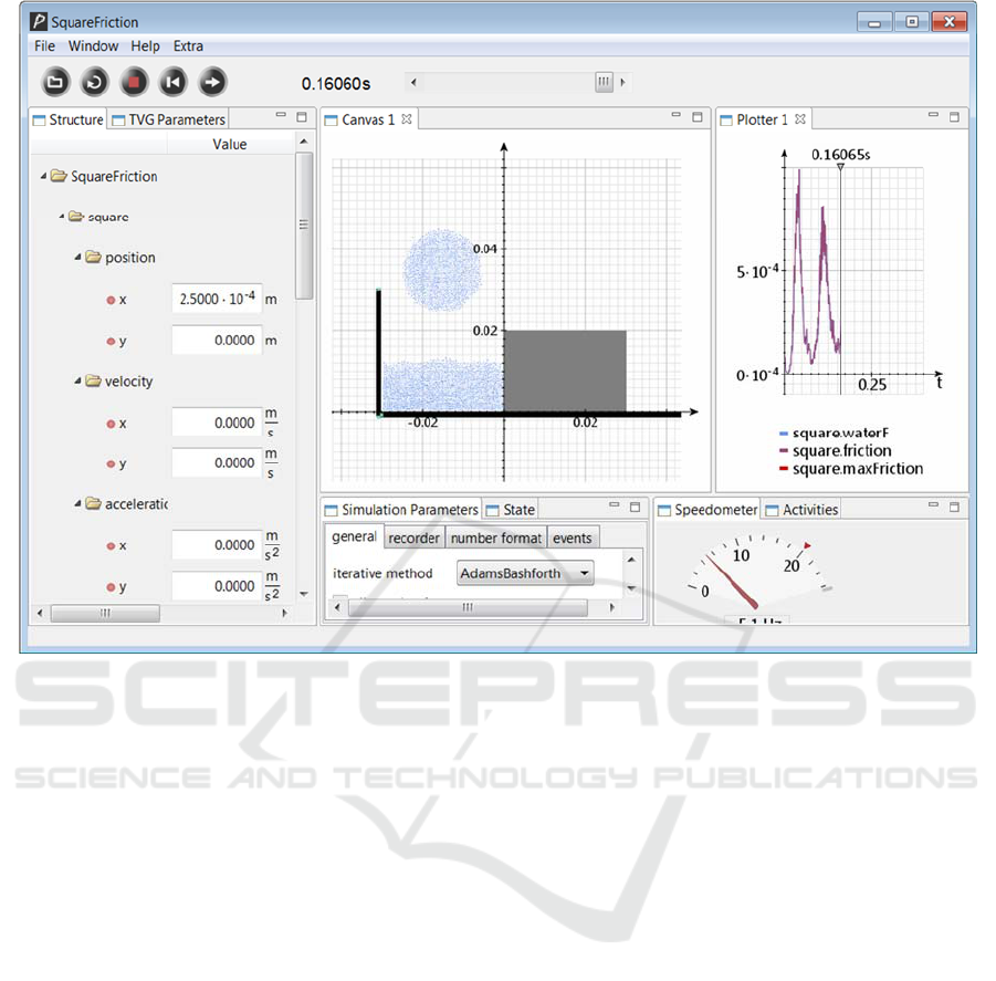
Figure 4: Physolator.

systems are implemented in a modular style, where a

physical system is built from components such as

point masses, springs, liquids etc.. Such components

are called physical components. They are defined as

Java classes. Each physical component represents a

part of a physical system with some physical

variables and formulas. Once you have defined such

components, you can reuse them in different

physical systems. In many cases, building a physical

system means just composing physical components:

build instances of the classes representing the

physical components, assign the variables of the

physical components appropriate values and link the

physical components together. Example: First create

some point masses, springs and pivot points. Then

assign appropriate constants to the physical

components: initial positions, masses, spring rates.

Finally, connect each end of a spring either with a

point mass or a pivot point.

Every physical system may have one or more

graphics components. Graphics components linked

to a physical system are automatically loaded

whenever the physical system is loaded. Graphics

components are used to visually represent the

current state of a physical system. During the

physical simulation, the variables of the physical

system change their values. A graphical

representation is easier to receive than a big number

of physical variable values. Therefore, graphics

components can be used to visually represent the

state of the physical system.

Graphics components are Java classes. For every

physical system one can implement a specific

graphics component tailored to this specific physical

system. The Physolator provides a means for

constructing generic graphical components. Generic

graphics components are tailored not to a single

physical system, but to a variety of physical systems

from a certain domain. They are reusable. Whenever

you implement a physical system for the specific

domain, you can simply use the generic graphics

component and you do not have to implement your

own graphics component.

4 THE FRB CLASS LIBRARY

The FRB library provides a set of physical

components plus some graphics components. Figure

5 shows the program code for the physical system

from section 2. Loading this piece of program to the

Physolator and starting the simulation results in the

Mixed Fluid and Rigid Body Simulations - An Object Oriented Component Library based on the Physolator Framework

1 public class SquareFriction extends MRBParticleSystem {

3 private final double sigma0 = 50e-5;

4 private final double rMax = 5 * sigma0;

5 private final Vector2D g = new Vector2D(0, -9.81);

6 private Line line =

7 new Line(new Vector2D(0.06, 0), new Vector2D(-0.03, 0));

8 public FrictionSquare square =

9 new FrictionSquare(0.00025, 0, 0.03, 0.02,line,0.6, 0.2);

11 public SquareFriction() {

12 beginStructure(rMax);

14 setParticleSchema(water, sigma0, g);

15 setMRBSchema(movableRigid, sigma0, g, square);

16 setRBSchema(rigid, sigma0);

18 line.schema = actualRBSchema;

19 addLine(-0.03, -0.001325, -0.03, 0.03);

20 addLine(line);

21 addMovableRigidBody(square);

23 fillRectangle(-0.02975,0.00025, 0, 0.015);

24 fillCircle(-0.015, 0.035, 0.01);

26 endStrukture();

27 }

29 public void initPlotterDescriptors(PlotterParameters r) {

30 r.add("square.acceleration.x, square.velocity.x",0.4, -1, 2);

31 r.add("square.F, square.friction",0.4, -1e-4, 10e-4);

32 }

33 }

Figure 5: Java program code.

simulation as shown in figure 1, figure 2 and figure

The program code from figure 5 defines a new

physical system named SquareFriction.

SquareFriction inherits from class

MRBParticleSystem. MRBParticleSystem is part of

the FRB library. It provides some features and

presets that make developing physical systems with

fluids and rigid bodies easier. Due to this inheritance

relationship, the physical system SquareFriction is

automatically equipped with appropriate default

values simulation parameters and it is automatically

equipped with a generic visualization component

tailored to the needs of fluid and rigid body

simulations. Figure 1 shows snapshots of this

component during the simulation.

The program code from figure 5 defines a

physical system by combining physical components

and by providing them with the right parameters and

settings. Lines 3 and 4 define the core parameters for

the particle model: sigma0 is used to specify the

particles equilibrium distance and rMax is a

constant, that defines a maximal distance. Forces

between two particles are neglected, if the distance

between the particles is greater than rMax (see

section 5 for details). Line 5 defines the earth

gravitation acceleration. Lines 6 through 9 define a

squared rigid body resting on a horizontal line. First,

the horizontal line is defined and then the squared

rigid body. Line 9 creates the squared rigid body.

The first four parameters define its location, width

and height. The fifth parameter is the previously

defined horizontal line. The squared rigid body has

an internal link to the horizontal line. Parameters six

and seven define the friction coefficients for static

friction and dry sliding friction, respectively.

The constructor of the class (lines 11 through 27)

defines the physical system. The commands that

build up the physical system are located between the

commands beginStructure and endStructure. Lines

14 through 16 initialize some data structures that are

used as containers for fluid bodies and rigid bodies,

respectively. See (Eisenbiegler, 2016b) for details.

Line 18 defines the standard behaviour of fluids, that

are in touch with rigid bodies. Lines 19 through 21

define three rigid bodies: two lines representing the

floor and the wall at the left hand side and a squared

block. The lines representing the floor and the wall

on the left hand side are rigid bodies, that are not

movable. The block is a movable rigid body. Lines

SIMULTECH 2017 - 7th International Conference on Simulation and Modeling Methodologies, Technologies and Applications

23 and 24 define amounts of water. Initially, the

basin is filled with a rectangular amount of water

and there is a circular amount of water located above

the basin.

Lines 30 and 31 define, that there shall be two

plots: one plot with the acceleration and the velocity

of the block and one plot with the force applied to

the block and the actual total friction. For every plot,

one has to define the names of the variables that are

to be displayed, the range of time and the minimal

and maximal values (y range).

To summarize, the program code of figure 5

defines a physical system by creating components

from given classes from the FRB library. The

program code creates some of these components,

provides them with the right parameters and

interconnects them. There are no physical formulas

in this program code. As a user of the FRB library,

you can just combine the components and you do

not have to think about the underlying physics. The

formulas representing the underlying physics are

located inside the physical components of the FRB

library.

5 EXAMPLES

The approach presented in the previous section can

be used to define different kinds of physical systems.

Figures 6 through 9 give some examples. All these

simulations have been implemented with the help of

the FRB library in the same style as program code in

figure 5.

I II

III IV

V VI

VII VIII

Figure 6: Example A.

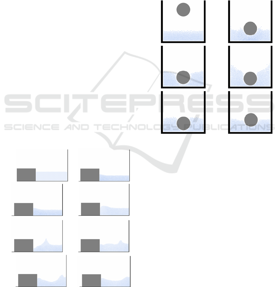
Figure 6 shows a physical system, that is similar

to the initial example from the previous section: a

basin with a block on one side and a fixed wall on

the opposite side. For a certain time, the block is

moved from left to right with a constant speed. Then

the block is stopped. As a result, the water inside the

basin starts moving. A wave moves from left to

right. When reaching the fixed wall on the right, the

wave is reflected and finally moves leftwards.

Figure 7 shows a ball, that is dropped into a

basin of water. As soon as the ball touches the water,

the water is pushed sideways and starts moving.

I II

III IV

V VI

Figure 7: Example B.

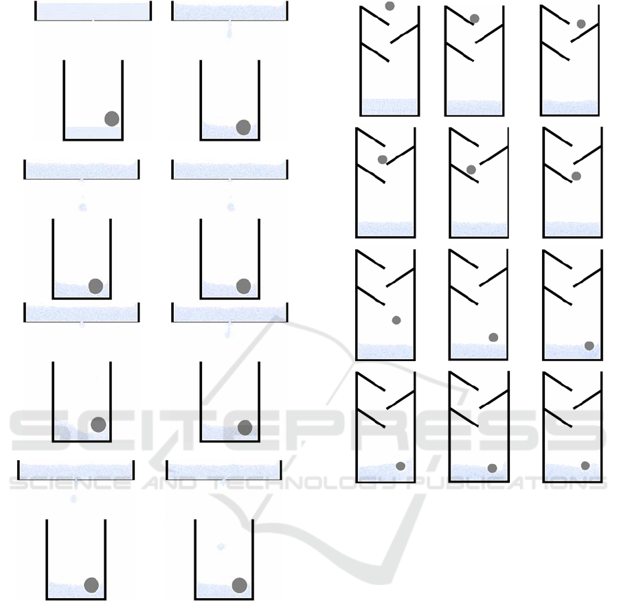
The physical system from figure 8 consists of

two basins of water. Due to a small hole in floor of

the upper basin, water drops from the upper basin to

the lower basin. The water drops falling into the

lower basin produce waves. In the lower basin, there

is a ball floating on the water. The waves move this

ball.

The physical system in figure 9 is similar to the

one from figure 7: a ball drops into a basin filled

with water. In figure 9, however, there are some

barriers. On its way down to the water, the ball hits

these barriers several time and rolls on them until it

finally plops into the water.

Mixed Fluid and Rigid Body Simulations - An Object Oriented Component Library based on the Physolator Framework

I II

III IV

V VI

VII VIII

Figure 8: Example C.

6 ALGORITHMIC

CONSIDERATIONS

The fluid simulation library from (Eisenbiegler,

2016b) provides a core infrastructure for modelling

pieces of fluid using particles. In a particle based

fluid simulation, the number of particles is crucial.

Theoretically, every particle interacts with every

other particle. For sake of simulation speed, a

maximum distance 



is defined. Forces between

particles are neglected if their distance is greater

than 



. A grid of boxes is used in order to effi-

I II III

IV V VI

VII VIII IX

X XI XII

Figure 9: Example D.

ciently find particles, that are in the neighbourhood

of some particle. The grid spacing is 



. Every

box inside this grid is quadratic with the width and

height being 



. All particles are assigned to

boxes in this grid. A hash map data structure is used

to efficiently find the neighbouring boxes. After

every movement of the particles, this data structure

is computed anew and all particles are assigned to

the boxes.

The FRB has been build on top of the fluid

simulation library (Eisenbiegler, 2016b). It provides

extra data structures for internally representing rigid

bodies. To achieve good results as to performance,

the algorithm for determining the particle-particle

forces has been enhanced using multi-threading.

Besides, an algorithm has been implemented for

efficiently determining the forces between particles

and rigid bodies.

In the fluid simulation library (Eisenbiegler,

2016b), a single threaded approach has been used to

determine the forces between the particles. When

SIMULTECH 2017 - 7th International Conference on Simulation and Modeling Methodologies, Technologies and Applications

working with several threads, one has to make sure,

that not more than one thread works with a particle

at the same time. To compute the forces for one

particle, one has to consider all particles from the

same box plus all the particles from the

neighbouring boxes. If two work with one particle at

the same time (reentrancy), this could lead to false

results. Synchronized methods would solve this

problem. However, they use locking and locking

could produce deadlocks. To synchronize the threads

and to avoid deadlocks, a specifically developed

synchronization strategy is to be used.

At a certain point in time every thread shall

determine the actual forces for all particles of some

box. To compute the forces of the particles in one

box, the thread also has to work with the particles

from the boxes in the direct neighbourhood. When

working with one box, no other thread shall work

with this box or its neighbours. If two threads are

determining the forces for two boxes, there must be

at least two boxes between these boxes.

Figure 10: Boxes used to avoid reentrancy.

Figure 10 explains the multi threading and

synchronization concept. In this figure, there are

several amounts of water. Each amount of water is

represented by a set of particles. During simulation,

an orthogonal grid of quadratic boxes is used and

each particle is assigned to one of the boxes. In

Figure 10, one can see vertical columns. Each

column represents a vertical sequence of boxes. The

width of the columns is 



. At a point in time, one

thread shall compute the forces for all particles of

one column plus the forces applied from these

particles to the particles that are in the columns next

to the actual column. One has to make sure, that at

no time there are two threads working with columns

with less than two columns in between. Figure 10

shows a snapshot during computation. The grey

columns represent columns, where a thread is

currently computing the forces.

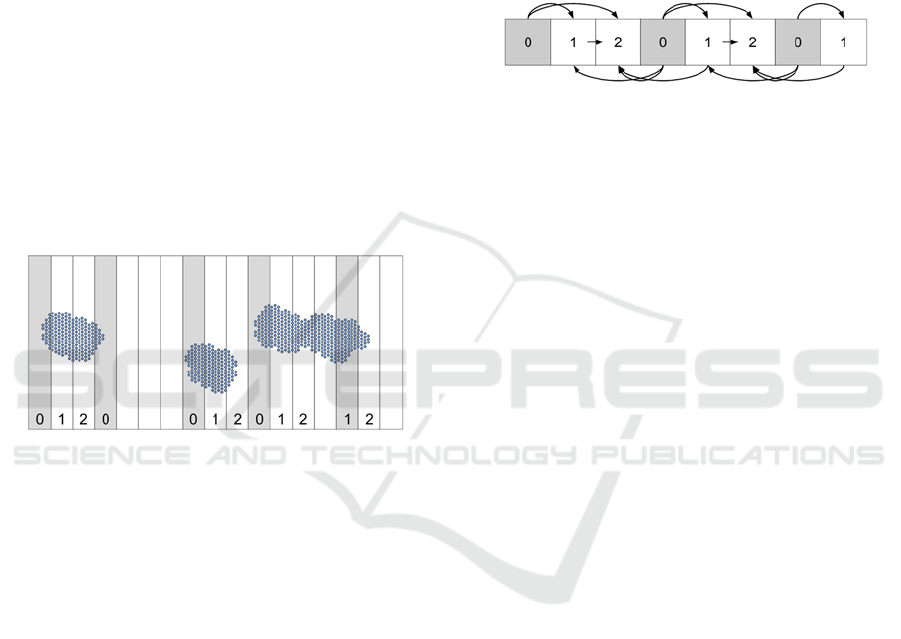
Threads are synchronized using the wait/notify

mechanism from Java to make sure, that at any time

there are at least two columns in between two active

threads. Figure 11 shows the pattern, that is used for

this synchronization. Each number represents one

column and each arrow represents a wait-notify-

relationship. The thread actually executing the

column at the starting point of the arrow has to

finish its work, unless the computation of the

column, that the arrow points to, cannot be started.

A thread at the end point of an arrow has to invoke

wait(). It is blocked unless the thread from the

starting point of the arrow sends him a notify()

signal.

Figure 11: Synchronization.

Rigid bodies are either represented by lines or by

circle segments. The algorithm shall compute all

forces, that particles apply to rigid bodies, and all

forces, that rigid bodies apply to particles.

Theoretically, one would have to consider all

combinations of rigid bodies and particles. To save

computing time, forces shall be neglected if the

distance is greater than 



The algorithms used for computing the forces

between rigid bodies and particles use the grid of

boxes. One has to find all combinations of boxes and

rigid bodies, where the box is not more than 



apart from the rigid body. More precisely: There is

at least one point inside the box, that is not more

than 



apart from the rigid body. For every such

pair of rigid body and box, one has to iterate through

all particles and compute the actual distance to the

rigid body. If the distance between the particle and

the rigid body is not greater than 



, then the force

between this particle and the rigid body is computed

and this force is added to the rigid body and to the

particle – with opposite signs.

But how to efficiently determine all

combinations of boxes and rigid bodies, that are not

more than 



apart? There are two different

approaches, that are to be called algorithm A and

algorithm B. Algorithm A iterates through all boxes.

For every box, the algorithm determines the distance

to all rigid bodies. Algorithm B works the other way

round: It iterates through all rigid bodies. For every

rigid body, the algorithm walks along the rigid body

from the beginning point to the end point of the line

and computes the position of the boxes in the

neighbourhood of the line. For every such position,

it checks, if there is such a box with particles.

Determining the position of all box positions is easy

for lines. Beginning at the starting point of the line,

one simply has to add a small piece of the direction

Mixed Fluid and Rigid Body Simulations - An Object Oriented Component Library based on the Physolator Framework

vector to iterate through all the boxes, that are in the

neighbourhood of the line. Things are a little trickier

with circle segments. To solve this problem, the

algorithm uses the Bresenham algorithm

(Bresenham, 1965). This algorithm has initially been

invented to draw circular lines using a plotter.

The user of the FRB library can choose between

algorithm A and algorithm B. The result is always

the same, but the computing efficiency is different.

It depends on the physical system, which of them is

faster. Algorithm A performs well for a smaller

number of particles and boxes and for a reasonable

number of rigid bodies. For a big number of

particles and a small number of rigid bodies with a

small total line length, algorithm B is faster.

7 CONCLUSIONS AND

OUTLOOK

This paper has presented a modular approach

towards mixed fluid and rigid body systems. So far,

there are still some limitations. First of all, the

approach is based on the fluid library presented in

(Eisenbiegler, 2016b) and this fluid library is limited

to two dimensional simulations. Three dimensional

fluid simulations are challenging. It takes far bigger

numbers of particles to achieve the same precision

with a three dimensional model. This results in a far

bigger amount of computing time.

The rigid body physics used in the examples is

limited to some physical effects: static friction,

dynamic friction, and collision. The library is so far

restricted to these effects. More physical effects

could be added and should be added.

So far, there has been a focus on optimizing the

fluid simulations. The data structures and algorithms

are optimized to handle as many fluid particles as

possible. However, the FRB library is not yet

designed for big numbers of rigid bodies.

REFERENCES

Eisenbiegler, D., 2015a. The Software Architecture of the

Physolator – a Physical Simulation Framework. In

MSAM 2015, Conference on Modelling, Simulation

and Appled Mathematics, Atlantis Press, pp. 61-64.

Eisenbiegler, D., 2016a. Object Oriented Modeling and

Simulation with the Physolator – Getting Started,

Available at: https://opus.hs-furtwangen.de/frontdoor/

index/index/docId/614.

Eisenbiegler, D., 2016b. A Generic Particle Modeling

Library for Fluid Simulation. In AMSM 2016,

Conference on Applied Mathematics, Simulation and

Modelling, Atlantis Press.

Eisenbiegler, D., 2015b. Objektorientierte Modellierung

und Simulation physikalischer Systeme mit dem

Physolator, BoD Norderstedt.

Eisenbiegler, D., 2016c. An Object Oriented Library for

Acoustics Simulation Based on the Physolator

Simulation Framework, In CMSAM 2016, Conference

on Modeling, Simulation and Applied Mathematics,

DEStech Publications.

Greenspan, D., 1997. Particle Modeling, Birkhäuser

Boston, Basel, Berlin.

Greenspan, D., 2004. N-Body Problems and Models,

World Scientific Publishing Co. Pte. Ltd.

Greenspan, D., 1985. Computer Studies in Particle

Modeling of Fluid Phenomena, Mathematical

Modeling, Vol. 6, pp 273-294, Pergamon Press Ltd..

Nijmeijer, M. J. P., et al., 1992. Molecular Dynamics of

the Surface Tension of a Drop, The Journal of

Chemical Physics, vol. 96, no. 1, pp. 565-576.

Korlie, M. S., 1997. Particle Modeling of Liquid Drop

Formation on a Solid Surface in 3-D, Elsevier Science

Ltd, Computers Math. Applic. Vol. 33, No. 9, pp. 97-

114.

Korlie, M. S., 1999. Three-Dimensional Computer

Simulation of Liquid Drop Evaporation, Computers &

Mathematics with applications, Elsevier.

Bresenham, J. E., 1965. Algorithm for computer control of

a digial plotter, IBM Systems Journal, Vol. 4, p. 24.

Pozrikidis, C., 2017. Fluid Simulation – Theory,

Computation, and Numerical Simulation”, Springer.

SIMULTECH 2017 - 7th International Conference on Simulation and Modeling Methodologies, Technologies and Applications