
Optical MIMO Multi-mode Fiber Transmission using Photonic Lanterns
Andreas Ahrens, André Sandmann and Steffen Lochmann
Hochschule Wismar, University of Applied Sciences: Technology, Business and Design,
Philipp-Müller-Straße 14, 23966 Wismar, Germany
Keywords:
Multiple-input Multiple-output Transmission, Optical MIMO, Photonic Lantern, Singular-value Decomposi-
tion.
Abstract:
Within the last years the multiple-input multiple-output (MIMO) technology has attracted increasing interest
in the optical fiber community. Theoretically, the concept of MIMO is well-understood and shows some
similarities to wireless MIMO systems. However, practical implementations of optical components are in the
focus of interest. Optical couplers have long been used as passive optical components being able to combine
or split single-input single-output (SISO) data transmissions. They have been proven to be well-suited for
the optical MIMO transmission despite their insertion losses and asymmetries. Nowadays, next to optical
couplers, photonic lanterns (PLs) have attracted a lot of attention in the research community as they offer the
benefit of a low loss transition from the input fibers to the modes supported by the waveguide at its output. In
this contribution the properties of a six-port PL are evaluated by measurements with regards to their respective
MIMO suitability. Based on the obtained results, a simplified time-domain MIMO simulation model, including
PLs for mode combining at the transmitter-side as well as for mode splitting at the receiver-side, is elaborated.
Our results obtained by the simulated bit-error rate (BER) performance as well as by measurements show that
PLs are well-suited for the optical MIMO transmission.
1 INTRODUCTION
The growing demand of bandwidth particularly
driven by the developing Internet has been satisfied
so far by optical fiber technologies such as dense
wavelength division multiplexing, polarization divi-
sion multiplexing and multi-level modulation. These
technologies have now reached a state of maturity
(Winzer, 2012). The only way to further increase
the available data rate is now be seen in the area of
spatial multiplexing (Richardson et al., 2013), which
is well-established in wireless communications (Tse
and Viswanath, 2005). Nowadays several novel tech-
niques such as mode group division multiplexing or
multiple-input multiple-output (MIMO) are in the fo-
cus of interest (Singer et al., 2008). Among these
techniques, the concept of MIMO transmission over
multi-mode fibers has attracted increasing interest in
the optical fiber transmission community, targeting at
increased fiber capacity (Foschini, 1996; Singer et al.,
2008; Winzer and Foschini, 2014). The fiber capac-
ity of a multi-mode fiber is limited by the modal dis-
persion compared to single-mode transmission where
no modal dispersion except for polarization exists. In
theory, the optical MIMO concept is well-described
(Singer et al., 2008). However, the practical realiza-
tion of the optical MIMO channel requires substan-
tial further research regardingmode combining, mode
maintenance and mode splitting (Schöllmann and
Rosenkranz, 2007; Schöllmann et al., 2008; Sand-
mann et al., 2016; Sandmann et al., 2014). Hence,
photonic lanterns (PLs) have attracted a lot of atten-
tion in the research community (Leon-Saval et al.,
2014). Compared to other passive devices used for
mode combining and mode splitting such as optical
couplers, PLs offer the benefit of a low loss transi-
tion from the input fibers to the modes supported by
the waveguide at its output which makes such devices
very attractive for optical MIMO communication.
Against this background, the novel contribution of
this paper is that based on measurements the suitabil-
ity of PLs for mode combining and splitting is studied
by computer simulations.
The remaining parts of this paper are structured
as follows: Section 2 introduces the studied optical
MIMO system based on PLs and shows measured
characteristics of a 6-port PL. Based on these charac-
teristics in section 3 a corresponding electrical MIMO
channel model is derived. The block-oriented and
SVD-based broadband MIMO system is described in
24
Ahrens, A., Sandmann, A. and Lochmann, S.
Optical MIMO Multi-mode Fiber Transmission using Photonic Lanterns.
DOI: 10.5220/0006394800240031
In Proceedings of the 14th International Joint Conference on e-Business and Telecommunications (ICETE 2017) - Volume 3: OPTICS, pages 24-31
ISBN: 978-989-758-258-5
Copyright © 2017 by SCITEPRESS – Science and Technology Publications, Lda. All rights reserved
section 4. The associated performance results are pre-
sented and interpreted in section 5. Finally, section 6
provides the concluding remarks.
2 OPTICAL MIMO
TRANSMISSION
One approach to form an optical MIMO system is
to transmit multiple data signals on different spa-
tial modes through a few-mode or multi-mode fiber
(FMF/ MMF). In this work, photonic lanterns (PLs)
are studied in order to transfer the binary information
carried on the LP
01
mode in n
T
single-mode fibers
(SMFs) to discrete modes in a FMF and vice versa.
The physical transmission model is depicted in Fig. 1.
The FMF carries n
M
modes depending on the geomet-
ric as well as the physical structure of the fiber and the
operating wavelength. Subsequent to the transmission
through a FMF of length ℓ, the modes are demulti-
plexed to n
R
SMFs with an inversely arranged PL.
In theory, for transitioning the incident modes of
the SMF to the respective modes carried in the few
mode fiber with low loss the condition n
T
= n
M
= n
R
needs to be respected (Leon-Saval et al., 2013). How-
ever, measurements of the transfer characteristic of
the fusion type PL with 6-ports shows quite a notice-
able insertion loss and slight asymmetries between the
different SMF inputs, see Tab. 1. Still, these asymme-
tries are relatively small when comparing to the in-
sertion loss differences of an optical MIMO system
based on offset SMF to MMF splices and fusion cou-
plers as shown in the same table (Sandmann et al.,
2016). Contrary to expectations, the photonic inte-
grated circuit (PIC) type 6-port PL shows the best re-
sults with respect to the insertion loss. Extending a
fusion coupler based system to 6-ports requires the
concatenation of multiple 2-port systems which is ac-
companied by a significant insertion loss increase.
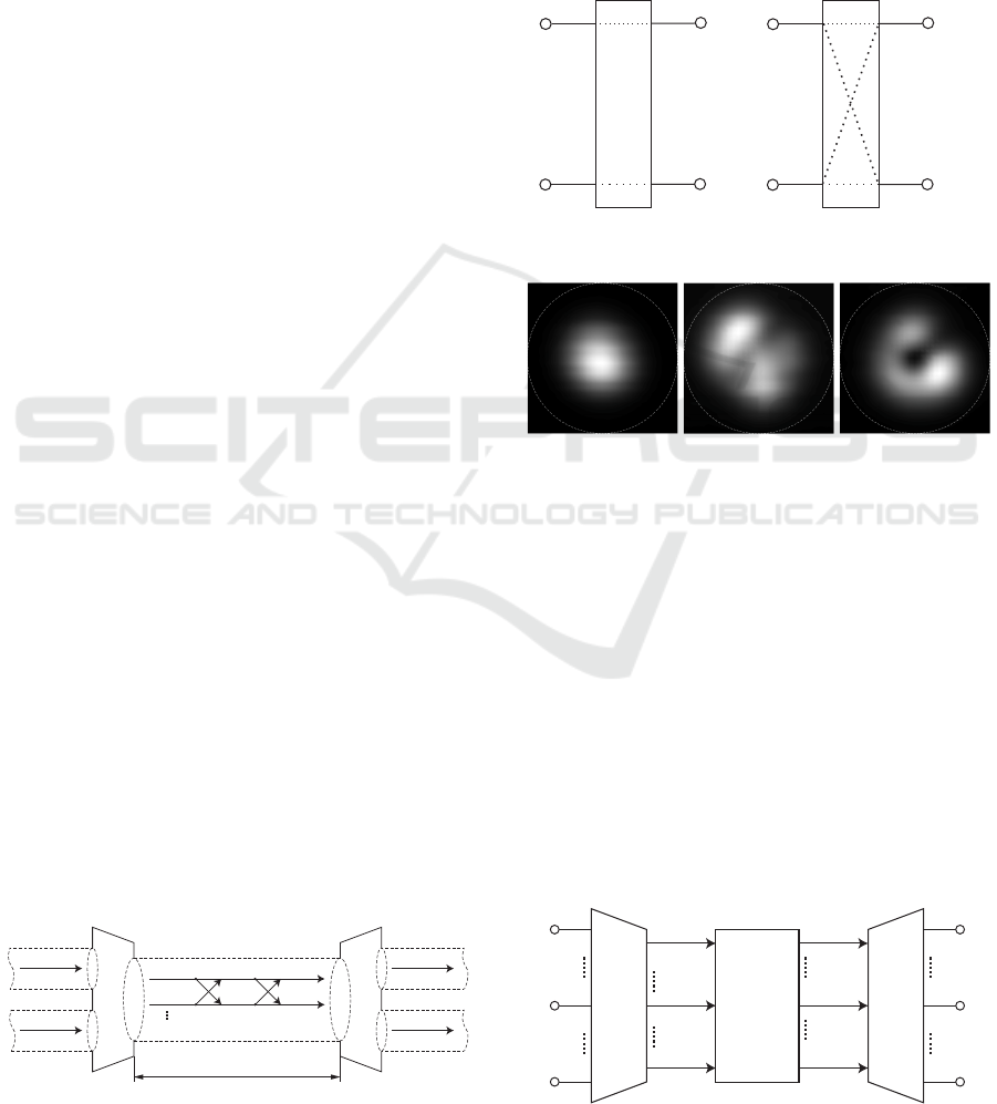
Considering the modal behavior, under ideal con-
ditions the PL transfers the signals from each SMF to
a discrete mode in the FMF, see Fig. 2. In contrast,
three spatial intensity patterns measured at the out-
put of the 6-port PL, compare Fig. 3, show that a real
PL excites a combination of modes which are super-
SMFsSMFs
FMF / MMF
LP
01
LP
01
LP
01
LP
01
LP
01
LP
11
Photonic Lantern
Photonic Lantern
ℓ
Figure 1: Multi-mode MIMO transmission model using
photonic lanterns for mode combining and splitting.
imposed in the FMF, e.g. the LP
01
and LP
11
modes.
This can be interpreted as cross-talk. In addition to
the cross-talk introduced by the PLs, mode mixing
during the transmission through the FMF occurs due
to micro bends etc. The idea is to apply MIMO sig-
nal processing in order to remove the cross-talk. For
this purpose, the transmission relations are described
in an electrical system model.
LP
01
LP
01
LP
01
LP
01
LP
01
LP
11
ideal
real
LP +LP +...
01 11
LP +LP +...
11 01
SMFs FMF SMFs FMF
Figure 2: Comparing the spatial mode transformation char-
acteristic of a real PL with an ideal PL.
Figure 3: Example of measured spatial intensity patterns at
the output of a fusion type PL using different input SMFs
at an operating wavelength of λ = 1550 nm; the dotted line
represents the 30 µm fiber core diameter.
3 ELECTRICAL MIMO
CHANNEL REPRESENTATION
The electrical baseband MIMO channel representa-
tion employing PLs and a FMF is shown in Fig. 4.
Here, the transmitter-side photonic lantern is fed by
the signals a
µ
(t), with µ = 1,..., n
T
, representing
the optical signals carried on the LP
01
mode in the
SMFs. Correspondingly, the signals b
β
(t) represent
the guided spatial modes at the input of the FMF
and c
κ
(t) are the resulting FMF output signals, where
Photonic Lantern
Photonic Lantern
FMF Channel
a
1
(t)
a
µ
(t)
a
n
T
(t)
d
1
(t)
d
ν
(t)
d
n
R
(t)
b
1
(t)
b
β
(t)
b
n
M
(t)
c
1
(t)
c
κ
(t)
c
n
M
(t)
Figure 4: Electrical MIMO channel model.
Optical MIMO Multi-mode Fiber Transmission using Photonic Lanterns
25
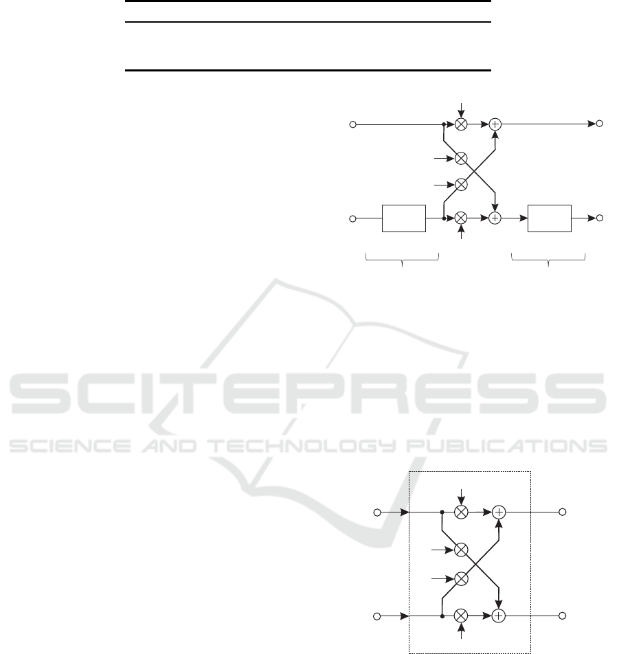
Table 1: Insertion loss measurements when launching from different SMF inputs through a fusion type and photonic integrated
circuit (PIC) type 6-port photonic lantern compared to a 2-port fusion coupler based system.
SMF input number 1 2 3 4 5 6
Fusion type PL insert. loss [dB] 6.7 6.7 4.2 4.1 7.0 4.1
PIC type PL insert. loss [dB] 1.7 2.2 1.5 2.2 2.0 1.7
Fusion coupler insert. loss [dB] 0.1 8.1 – – – –
β,κ = 1,.. .,n
M
. Finally, the receiver-side PL trans-
fers the modes of the FMF to fundamental modes
in the SMFs, represented by the signals d
ν
(t), with
ν = 1,. .. ,n
R
. For simplification purposes and in
order to create the prerequisites for a near lossless
transmission the number of input SMFs n
T
, the num-
ber of guided modes in the FMF n
M
and the num-
ber of output SMFs n
R
are assumed to be identi-
cally. In this work, these numbers are chosen to be
n
T
= n
M
= n
R
= 2 and therefore only the LP
01
and
LP
11
modes can propagate implying a V-number in
range 2.405 < V < 3.832 when transmitting through
a step-index profiled FMF. The degenerate modes of
LP
11
, i.e. LP
11a
and LP
11b
, are summarized.
3.1 FMF Channel
The transmission properties of the FMF are repre-
sented by the model depicted in Fig. 5. In time-
domain, the system characteristics of the FMF chan-
nel are given as follows
c
1
(t) = k
(CH)
11
b
1
(t) + k
(CH)
12
b
2
(t − ∆τ/2)
c
2
(t) = k
(CH)
21
b
1
(t − ∆τ/2) + k
(CH)
22
b
2
(t − ∆τ) ,
(1)
describing the mode-coupling of the underlying chan-
nel. Herein, the parameter ∆τ describes the differen-
tial mode delay between the fundamental mode LP
01
and the mode LP
11
, which is identified to be ∆τ =
200 ps for the considered fiber length of ℓ = 2 km.
The effect of the chromatic dispersion is not ana-
lyzed in this contribution since a zero chromatic dis-
persion wavelength is assumed which is in the region
of 1300 nm. However, for different wavelengths chro-
matic dispersion can be taken into account by a sim-
ple convolution with a Gaussian function. The optical
field coupling coefficients k
(CH)
κβ
describe the coupling
from the mode LP
01
to the mode LP
11
, from the mode
LP
11
to the mode LP
01
and so forth. Since a lossless
transmission through the FMF is assumed, the cou-
pling coefficients have to fulfill the following condi-
tion
n
M
∑
κ=1
k
(CH)
κβ
2
= 1 ∀ β . (2)
. Finally, the receiver-side PL trans-
fers the modes of the FMF to fundamental modes
, with
. For simplification purposes and in
order to create the prerequisites for a near lossless
, the num-
and the num-
are assumed to be identi-
cally. In this work, these numbers are chosen to be
and
modes can propagate implying a V-number in
832 when transmitting through
a step-index profiled FMF. The degenerate modes of
b
1
(t)
c
1
(t)
b
2
(t)
c
2
(t)
ℓ/2
ℓ/2
∆τ/2
∆τ/2
k
(CH)
1 1
k
(CH)
2 2
k
(CH)
2 1
k
(CH)
1 2
Figure 5: Underlying FMF channel model of length de-
Figure 5: Underlying FMF channel model of length ℓ de-
signed for two mode propagation (n
M
= 2).
3.2 Photonic Lanterns
Hereinafter, the mode combining and mode splitting
process conducted by the photonic lanterns is studied.
Considering a (2× 2) PL the corresponding electrical
representation for the transmitter-side PL is shown in
Fig. 6. At the transmitter-side the mapping of the
a
1
(t)
b
1
(t)
a
2
(t)
b
2
(t)
k
(PL,TX)
1 1
k
(PL,TX)
2 2
k
(PL,TX)
2 1
k
(PL,TX)
1 2
Figure 6: Electrical system model of the transmitter-side PL
(n
T
= n
M
= 2).
incident LP
01
modes, represented by the signals a
µ
(t),
by the PL can be described with the corresponding
coupling matrix
K
(TX)
=
k
(PL,TX)
11
· · · k
(PL,TX)
1n
T
.
.
.
.
.
.
.
.
.
k
(PL,TX)
n
M
1
· · · k
(PL,TX)
n
M
n
T
, (3)
OPTICS 2017 - 8th International Conference on Optical Communication Systems
26
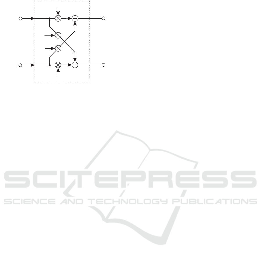
c
1
(t)
d
1
(t)
c
2
(t)
d
2
(t)
k
(PL,RX)
1 1
k
(PL,RX)
2 2
k
(PL,RX)
2 1
k
(PL,RX)
1 2
Figure 7: Electrical system model of the receiver-side PL
(n
M
= n
R
= 2).
with k
(PL,TX)
βµ
denoting the transmitter-side coupling
coefficients. Having an ideal PL, compare Fig. 2,
the coupling matrix is given by an identity matrix
considering n
M
= n
T
. Since the receiver-side PL is
inversely arranged and is assumed to have identi-
cal properties to the transmitter-side PL, the corre-
sponding coupling matrix is the transpose denoted
by (· )
T
of the transmitter-side coupling matrix, i.e.
K
(RX)
=
K
(TX)
T
. Here, it is worth noting that un-
der practical assumptions the output LP
01
modes of
the receiver-side PL appear as superpositions of the
LP
01
and LP
11
modes of the FMF as highlighted in
Fig. 2. Having a non-ideal PL, the corresponding
electrical system model is shown in Fig. 7 for the
receiver-side PL. Here, k
(PL,RX)
νκ
denotes the receiver-
side coupling coefficients, being summarized in the
coupling matrix K
(RX)
. Based on the short fiber
length, the PL is assumed to be flat in the considered
frequency band. Since no power-loss is assumed, the
transmitter-side PL coupling coefficients are required
to comply to
n
M
∑
β=1
k
(PL,TX)
βµ
2
= 1 for µ = 1, ... ,n
T
(4)
and the receiver-side PL coupling coefficients need to
fulfill the following condition
n
R
∑
ν=1
k
(PL,RX)
νκ
2
= 1 for κ = 1,..., n
M
. (5)
Considering the overall MIMO channel model,
compare Fig. 4, as a black box with two in- and out-
puts the transfer characteristic can be described by the
corresponding MIMO impulse responses g
νµ
(t). In-
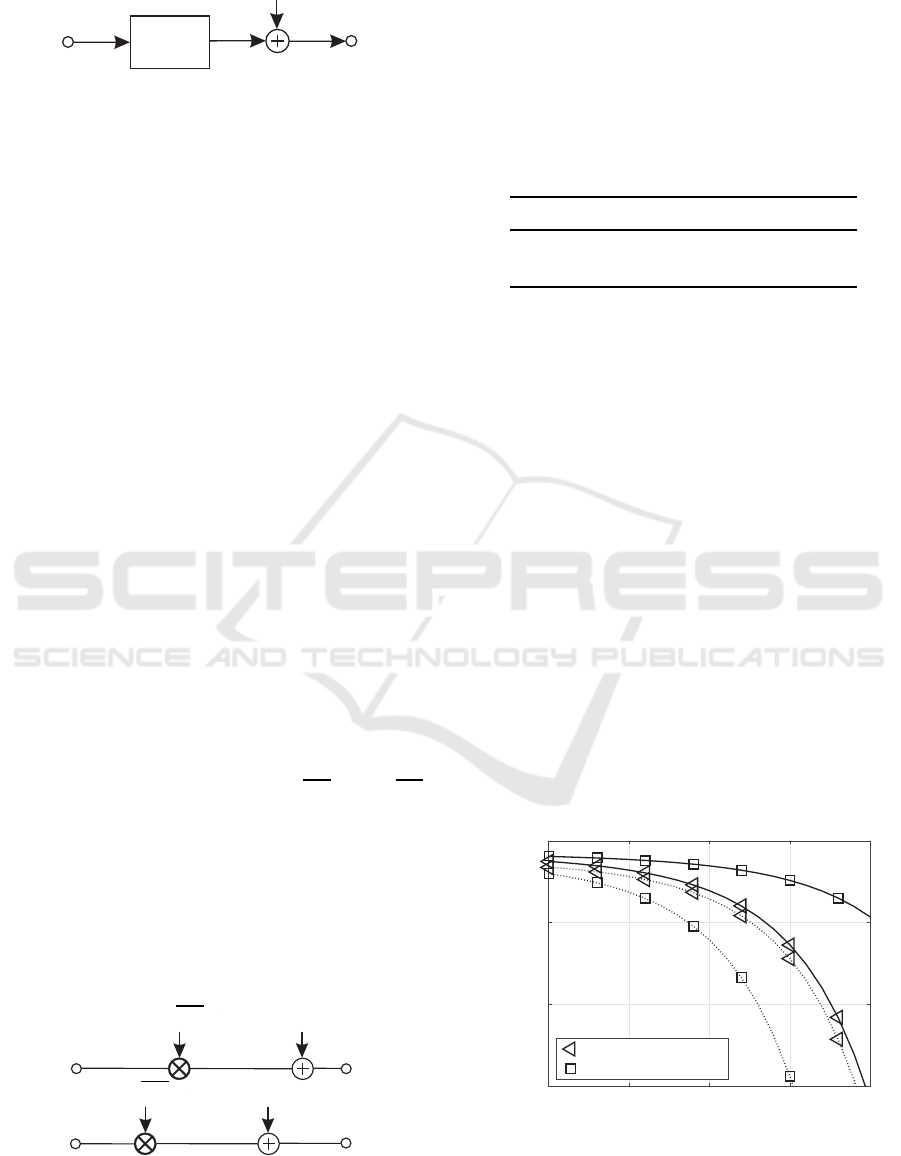
cluding pulse shaping and receive filtering function-
ality the overall (2× 2) MIMO transmission model is
depicted in Fig. 8. Rectangular pulses of frequency
f
T
= 1/T
s
are used for pulse shaping and receive fil-
tering, i.e. g
s
(t) and g
ef
(t) and hence the overall im-
pulse responses h
νµ
(t) are formed as follows
h
νµ
(t) = g
s
(t) ∗ g
νµ
(t) ∗ g
ef
(t) , (6)
where ∗ denotes the convolution operator. An ad-
ditional component to be considered is the additive
white Gaussian noise (AWGN) denoted by the term
en
ν
(t). The sampled overall impulse responses are
used for the broadband MIMO system model, being
described in the next section.
4 BROADBAND MIMO SYSTEM
DESCRIPTION
Considering a frequency-selective MIMO link, com-
posed of n
T
optical inputs and n
R
optical outputs, the
resulting electrical discrete-time block-oriented sys-
tem is modeled referring to (Raleigh and Cioffi, 1998;
Pankow et al., 2011) as follows
u = H· b+ n . (7)
Vector b of size (N
T
× 1) contains the input symbols
transmitted over n
T
optical inputs in K consecutive
time slots, i.e. N
T
= K n
T
. This vector can be decom-
posed into n
T
input-specific signal vectors b
µ
accord-
ing to
b =
b
T
1
,.. ., b
T
µ
,.. ., b
T
n
T
T
, (8)
where (· )
T
denotes the transpose operator. These
input-specific signal vectors of size (K × 1) include
the symbols transmitted at the optical input µ for all
time instances k, with k = 1,. .. ,K, as given by
b
µ
=
b
1µ
,.. ., b
kµ
,.. ., b
Kµ
T
. (9)
The (N
R
× 1) sized received signal vector u can again
be decomposed into n
R
output-specific signal vectors
u
ν
of the length K + L
c
, i. e. N
R
= (K + L
c
)n
R
, and
results in
u =
u
T
1
,.. ., u
T
ν
,.. .,u
T
n
R
T
. (10)
By taking the (L
c
+ 1) non-zero elements of the re-
sulting symbol rate sampled overall channel impulse
response h
νµ
(t) between the µth input and νth out-
put into account, the output-specific received vector
u
ν
has to be extended by L
c
elements, compared to
the transmitted input-specific signal vector b
µ
defined
in (9). The ((K + L
c
) × 1) signal vector u
ν
received
by the optical output ν can be constructed, including
the extension through the multi-path propagation, as
follows
u
ν
=
u
1ν
,u
2ν
,.. ., u
(K+L
c
)ν
T
. (11)
Optical MIMO Multi-mode Fiber Transmission using Photonic Lanterns
27
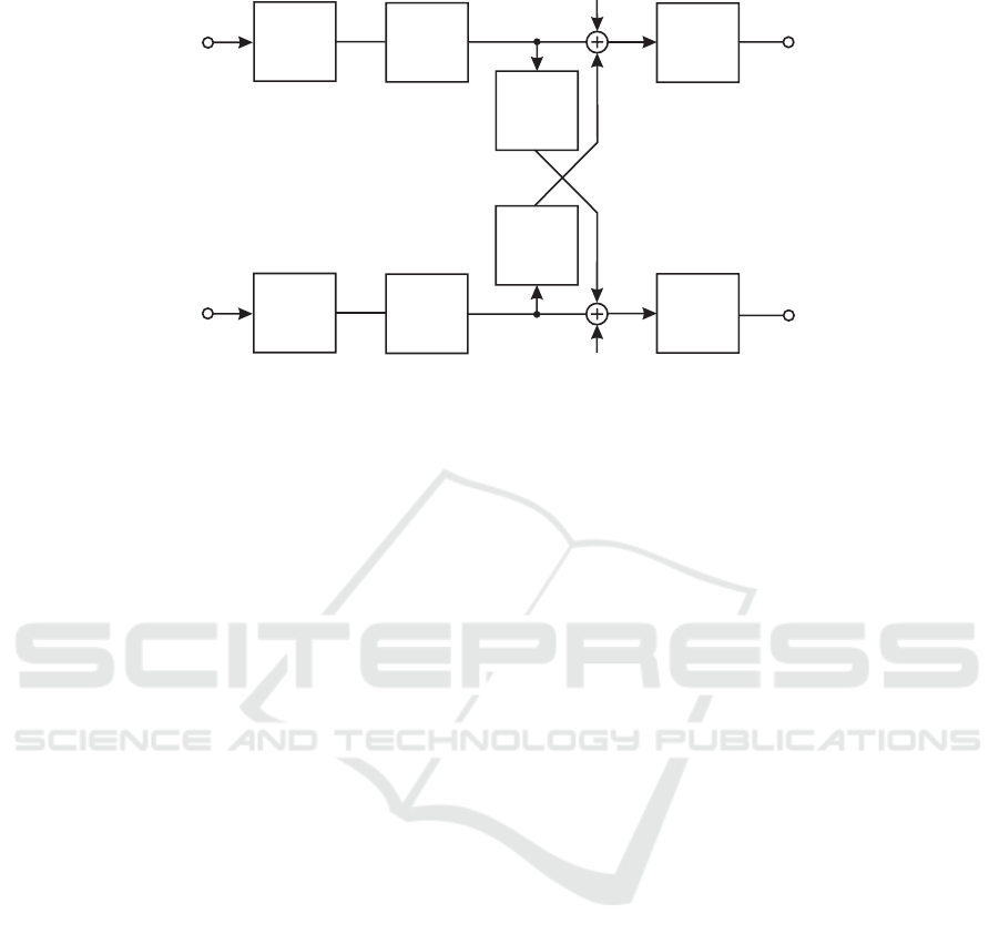
s
1
(t)
s
2
(t)
a
1
(t)
a
2
(t)
d
1
(t)
d
2
(t)
r
1
(t)
r
2
(t)
g
s
(t)
g
s
(t)
g
ef
(t)
g
ef
(t)
g
11
(t)
g
21
(t)
g
12
(t)
g
22
(t)
e
n
1
(t)
e
n
2
(t)
Figure 8: Electrical (2× 2) MIMO transmission model.
Correspondingly, the (N
R
× 1) sized vector n de-
notes the AWGN after receive filtering with g
ef
(t)
and sampling. Finally, the (N
R
× N
T
) sized system
matrix H of the block-oriented system model de-
scribes the symbol rate sampled overall MIMO chan-
nel h
νµ
(t) consisting of the frequency-flat transmitter-
and receiver-side PL models as well as the frequency-
selective FMF model, the transmit and receive filter.
The channel matrix H is composed as follows
H = H
(RX)
· H
(CH)
· H
(TX)
. (12)
Herein, the (n
M
(K + L
c
) × n
M
K) sized matrix H
(CH)
describes the frequency-selective representation of
the FMF channel, compare Fig. 5, being structured
as follows
H
(CH)
=
H
(CH)
11
... H
(CH)
1n
M
.
.
.
.
.
.
.
.
.
H
(CH)
n
M
1
· · · H
(CH)
n
M
n
M
(13)
and consists of n
M
n
M
single-input single-output
(SISO) channel matrices H
(CH)
κβ
. Every of these ma-
trices H
(CH)
κβ
of the size ((K + L
c
) × K) describes the
L
c
+ 1 non-zero elements of resulting symbol rate
sampled impulse response of the FMF channel repre-
sentation including transmit and receive filtering, re-
sulting in:
H
(CH)
κβ
=
h
κβ
[0] 0 · · · 0
h
κβ
[1] h
κβ
[0] · · · 0
h
κβ
[2] h
κβ
[1] · · · 0
.
.
.
.
.
.
.
.
.
.
.
.
h
κβ
[L
c
] h
κβ
[L
c
− 1] · · ·
0 h
κβ
[L
c
] · · ·
.
.
.
.
.
.
.
.
.
.
.
.
0 0 ·· · h
κβ
[L
c
]
.
(14)
Since the transmitter-side photonic lantern (PL) is as-
sumed to be frequency-flat it can be described by a
((n
M
K)× (n
T
K)) pre-processing matrix
H
(TX)
= K
(TX)
⊗ I
K
, (15)
where ⊗ denotes the Kronecker product, K
(TX)
is
the transmitter-side PL coupling matrix and I
K
de-
fines a (K × K) identity matrix. Matrix H
(TX)
is com-
posed of concatenated (K × K) sized diagonal matri-
ces weighted by the corresponding coupling factors
k
(PL,TX)
βµ
. Correspondingly the receiver-side PL can
be described by a (n
R
(K + L
c
) × n
M
(K + L
c
)) post-
processing matrix
H
(RX)
= K
(RX)
⊗ I
K+L
c
, (16)
with K
(RX)
denoting the receiver-side PL coupling
matrix. The interference, which is introduced by the
off-diagonal elements of the channel matrix H, re-
quires appropriate signal processing strategies.
The MIMO block diagram of the transmission
model is shown in Fig. 9. A popular technique is
based on the singular-value decomposition (SVD) of
the system matrix H, which can be written as
H = S· V· D
H
, (17)
OPTICS 2017 - 8th International Conference on Optical Communication Systems
28
transmit vector
receive vector
noise vector
b
u
H
n
Figure 9: Transmission system model.
where S and D
H
are unitary matrices and V is a real-
valued diagonal matrix of the positive square roots
of the eigenvalues of the matrix H
H
H sorted in de-
scending order. In order to remove the interferences
pre-processed symbols b = D· c are transmitted, with
vector c denoting the unprocessed transmit symbols.
In turn, the receiver multiplies the received vector u
by the matrix S
H
. Thereby,neither the transmit power
nor the noise power is enhanced. The overall trans-
mission relationship is defined as
y = S
H
(H· D· c+ n) = V· c+ w. (18)
As a consequence of the processing in (18), the
channel matrix H is transformed into independent,
non-interfering layers having unequal gains (Pankow
et al., 2011; Raleigh and Cioffi, 1998; Ahrens and
Benavente-Peces, 2009). In MIMO communication,
singular-value decomposition (SVD) has been estab-
lished as an efficient concept to compensate the inter-
ferences between the different data streams transmit-
ted over a dispersive channel: SVD is able to transfer
the whole system into independent, non-interfering
layers exhibiting unequal gains per layer as high-
lighted in Fig. 10, where as a result weighted AWGN
channels appear.
Analyzing the considered (2× 2) MIMO system,
the data symbols at the time k, i. e. c
1k
and c
2k
are
weighted by the positive square roots of the eigen-
values of the matrix H
H
H, i.e.
p
ξ
1k
and
p
ξ
2k
.
The terms w
1k
and w
2k
denote the noise subsequent
to the SVD post-processing. It is worth noting that
the number of readily separable layers is limited by
min(n
T
,n
R
). Therefore, in this work the maximum
number of layers is given by L = 2. Based on this
non-interfering layer-specific transmission model the
bit-error rate performance can be calculated (Proakis,
2000).
p
ξ
1 k
p
ξ
2 k
w
1 k
w
2 k
c
1 k
c
2 k
y
1 k
y
2 k
Figure 10: SVD-based layer-specific transmission model.
5 PERFORMANCE RESULTS
In this section the BER quality, transmitting through
the (2 × 2) MIMO channel employing PLs for
mode combining and splitting, is studied using fixed
transmission modes with a spectral efficiency of
4 bit/s/Hz. The analyzed quadrature amplitude modu-
lation (QAM) constellations are listed in Tab. 2. This
Table 2: Transmission modes.
Spectral Efficiency Layer 1 Layer 2
4 bit/s/Hz 16 0
4 bit/s/Hz 4 4
bit allocation approach is combined with a power allo-
cation method that equalizes the signal-to-noise ratios
on all layers and time instances k in a data block for
optimizing the BER performance (Sandmann et al.,
2015).
In order to compare the performance of ideal PLs
to real PLs different cross-talk parameters have been
considered relating to the above described electrical
MIMO channel model. Since both PLs are assumed
to have identical properties in both directions and are
also assumed to be symmetric the PL cross-talk pa-
rameter is defined as follows
p
(PL)
cross
=
k
(PL,TX)
12
2
=
k
(PL,TX)
21
2
=
k
(PL,RX)
12
2
=
k
(PL,RX)
21
2
,
(19)
describing the electrical power transfer. The few-
mode fiber channel cross-talk is assumed to be sym-
metric as well as defined by
p
(CH)
cross
=
k
(CH)
12
2
=
k
(CH)
21
2
. (20)
denote the noise subsequent
to the SVD post-processing. It is worth noting that
the number of readily separable layers is limited by
. Therefore, in this work the maximum
2. Based on this
non-interfering layer-specific transmission model the
bit-error rate performance can be calculated (Proakis,
0 5 10 15 20
10
-6
10
-4
10
-2
10
0
10 · log
10
(E
s
/N
0
) (indB) →
BER →
ideal PL p
(PL)
cross
= 0
real PL p
(PL)
cross
= 0.1
Figure 11: BER performance when transmitting with the
Figure 11: BER performance when transmitting with the
(16,0) QAM constellation (dotted lines) and the (4,4) QAM
constellation (solid lines) assuming 10% FMF cross-talk,
i.e. p
(CH)
cross
= 0.1, at a symbol frequency of f
T
= 1 GHz.
Optical MIMO Multi-mode Fiber Transmission using Photonic Lanterns
29
0 5 10 15 20
10
-6
10
-4
10
-2
10
0
10 · log
10
(E
s
/N
0
) (indB) →
BER →
ideal PL p
(PL)
cross
= 0
real PL p
(PL)
cross
= 0.1
Figure 12: BER performance when transmitting with the
Figure 12: BER performance when transmitting with the
(16,0) QAM constellation (dotted lines) and the (4,4) QAM
constellation (solid lines) assuming 30% FMF cross-talk,
i.e. p
(CH)
cross
= 0.3, at a symbol frequency of f
T
= 1 GHz.
0 5 10 15 20
10
-6
10
-4
10
-2
10
0
10 · log
10
(E
s
/N
0
) (indB) →
BER →
ideal PL p
(PL)
cross
= 0
real PL p
(PL)
cross
= 0.1
Figure 13: BER performance when transmitting with the
Figure 13: BER performance when transmitting with the
(16,0) QAM constellation (dotted lines) and the (4,4) QAM
constellation (solid lines) assuming 30% FMF cross-talk,
i.e. p
(CH)
cross
= 0.3, at a symbol frequency of f
T
= 5 GHz.
The calculated BER results as a function of the
signal energy to noise power spectral density E
s
/N
0
are depicted in Fig. 11, 12 and 13 for different FMF
cross-talk parameter choices, i.e. p
(CH)
cross
, and sym-
bol frequencies f
T
. In all simulations the number
of symbols per data block and per layer is selected
to be K = 15. Choosing the (16,0) QAM constel-
lation shows the best BER performance results for
all configurations considering a real PL. The addi-
tional cross-talk introduced by a real PL increases the
MIMO channel correlation and thus the amplitude ra-
tio comparing the singular values of the two layers
increases as well. Therefore, the (16,0) QAM scheme
benefits from the additional cross-talk. In contrast,
the increased asymmetry of singular values impairs
the BER performance choosing the (4,4) QAM con-
stellation as highlighted by the results.
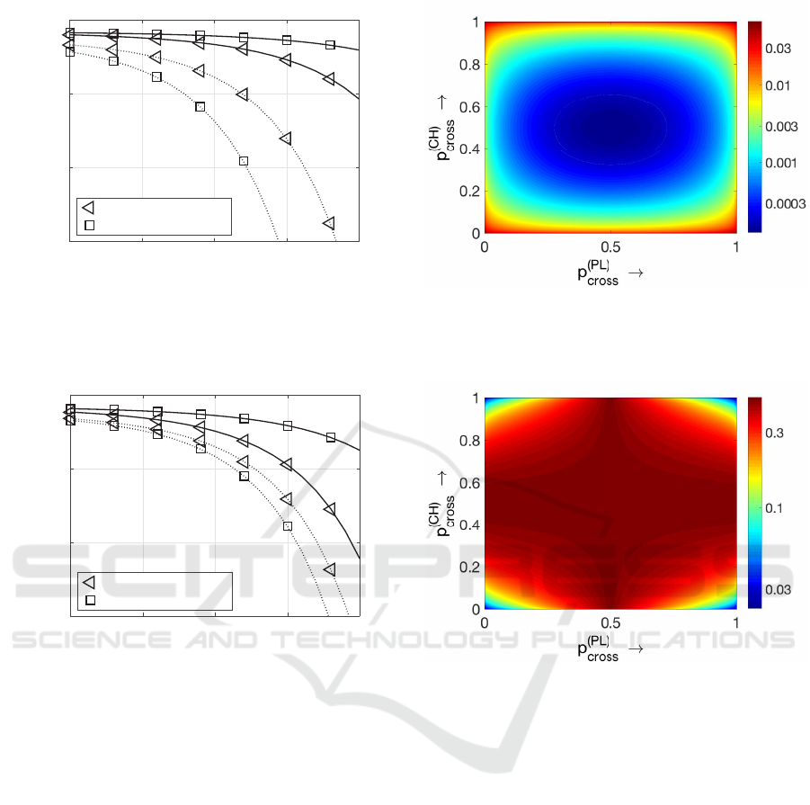
Figure 14: BER performance comparing different cross-talk
parameter choices when transmitting with the (16,0) QAM
constellation at a fixed E
s
/N
0
ratio of 10 dB at a symbol
frequency of f
T
= 1 GHz.
Figure 15: BER performance comparing different cross-talk
parameter choices when transmitting with the (4,4) QAM
constellation at a fixed E
s
/N
0
ratio of 10 dB at a symbol
frequency of f
T
= 1 GHz.
A second study shows the achievedBERs compar-
ing different cross-talk parameter choices, i.e. p
(CH)
cross
and p
(PL)
cross
, for the (16,0) QAM constellation in Fig. 14
and for the (4,4) QAM scheme in Fig. 15 at a fixed
E
s
/N
0
ratio of 10 dB. This study confirms that the
(16,0) QAM constellation benefits from high cross-
talk values whereas the (4,4) QAM constellation
shows a contrary behavior. It should be noted that
0.5 for p
(CH)
cross
as well as for p
(PL)
cross
is the value where
the most cross-talk is introduced into the system. All
in all, the best BER results are achieved with the
(16,0) QAM constellation in combination with high
cross-talk values when considering the studied simu-
lation environment.
OPTICS 2017 - 8th International Conference on Optical Communication Systems
30

6 CONCLUSIONS
In this contribution photonic lanterns as a mode cou-
pling and splitting device have been analyzed with
regard to their respective MIMO suitability. The es-
tablished time-domain MIMO simulation model has
been proven to be a versatile tool for the optimization
of the overall MIMO transmission performance. It
has been shown that the excitation of different mode
combinations by the PL, which has been interpreted
as cross-talk, does not impair the transmission qual-
ity. In certain constellations this cross-talk can help to
increase the BER performance. All in all, PLs seem
to be well-suited for optical MIMO communication
systems.
ACKNOWLEDGEMENTS
This work has been funded by the German Ministry
of Education and Research (No. 03FH016PX3).
REFERENCES
Ahrens, A. and Benavente-Peces, C. (2009). Modulation-
Mode and Power Assignment in Broadband MIMO
Systems. Facta Universitatis (Series Electronics and
Energetics), 22(3):313–327.
Foschini, G. J. (1996). Layered Space-Time Architecture
for Wireless Communication in a Fading Environment
when using Multi-Element Antennas. Bell Labs Tech-
nical Journal, 1(2):41–59.
Leon-Saval, S. G., Argyros, A., and Bland-Hawthorn, J.
(2013). Photonic lanterns. Nanophotonics, 2:429–
440.
Leon-Saval, S. G., Fontaine, N. K., Salazar-Gil, J. R., Er-
can, B., Ryf, R., and Bland-Hawthorn, J. (2014).
Mode-selective photonic lanterns for space-division
multiplexing. Opt. Express, 22(1):1036–1044.
Pankow, J., Aust, S., Lochmann, S., and Ahrens, A. (2011).
Modu-lation-Mode Assignment in SVD-assisted Op-
tical MIMO Multimode Fiber Links. In 15th Inter-
national Conference on Optical Network Design and
Modeling (ONDM), Bologna, Italy.
Proakis, J. G. (2000). Digital Communications. McGraw-
Hill, Boston.
Raleigh, G. G. and Cioffi, J. M. (1998). Spatio-Temporal
Coding for Wireless Communication. IEEE Transac-
tions on Communications, 46(3):357–366.
Richardson, D. J., Fini, J., and Nelson, L. (2013). Space
Division Multiplexing in Optical Fibres. Nature Pho-
tonics, 7:354–362.
Sandmann, A., Ahrens, A., and Lochmann, S. (2014). Ex-
perimental Description of Multimode MIMO Chan-
nels utilizing Optical Couplers. In Photonic Networks;
15. ITG Symposium; Proceedings of, pages 1–6.
Sandmann, A., Ahrens, A., and Lochmann, S. (2015).
Power Allocation in PMSVD-based Optical MIMO
Systems. In Advances in Wireless and Optical
Communications (RTUWO), pages 108–111, Riga
(Latvia).
Sandmann, A., Ahrens, A., and Lochmann, S. (2016). Ex-
perimental Evaluation of a (4x4) Multi-Mode MIMO
System Utilizing Customized Optical Fusion Cou-
plers. In ITG-Fachbericht 264: Photonische Netze,
pages 101–105, Leipzig (Germany). VDE VERLAG
GmbH.
Schöllmann, S. and Rosenkranz, W. (2007). Experimen-
tal Equalization of Crosstalk in a 2 x 2 MIMO Sys-
tem Based on Mode Group Diversity Multiplexing in
MMF Systems @ 10.7 Gb/s. In Optical Communi-
cation (ECOC), 2007 33rd European Conference and
Ehxibition of, pages 1–2.
Schöllmann, S., Schrammar, N., and Rosenkranz, W.
(2008). Experimental Realisation of 3 x 3 MIMO Sys-
tem with Mode Group Diversity Multiplexing Limited
by Modal Noise. In Optical Fiber Communication
Conference/National Fiber Optic Engineers Confer-
ence (OFC/NFOEC), pages 1–3.
Singer, A. C., Shanbhag, N. R., and Bae, H. M. (2008).
Electronic Dispersion Compensation - An Overview
of Optical Communications Systems. IEEE Signal
Processing Magazine, 25(6):110–130.
Tse, D. and Viswanath, P. (2005). Fundamentals of Wireless
Communication. Cambridge, New York.
Winzer, P. (2012). Optical Networking beyond WDM.
IEEE Photonics Journal, 4:647–651.
Winzer, P. J. and Foschini, G. J. (2014). Optical MIMO-
SDM system capacities. In Optical Fiber Commu-
nications Conference and Exhibition (OFC), 2014,
pages 1–3.
Optical MIMO Multi-mode Fiber Transmission using Photonic Lanterns
31
