
Unsupervised Segmentation of Nonstationary Data using Triplet Markov
Chains
Mohamed El Yazid Boudaren
1
, Emmanuel Monfrini
2
, Kadda Beghdad Bey
1
, Ahmed Habbouchi
1
and Wojciech Pieczynski
2
1
Ecole Militaire Polytechnique, PO Box 17, Bordj EL Bahri, Algiers 16111, Algeria
2
SAMOVAR, T
´
el
´
ecom SudParis, CNRS, Universit
´
e Paris-Saclay, 91011 Evry Cedex, France
{
Keywords:
Data Segmentation, Hidden Markov Chains, Nonstationary Data, Signal Processing, Triplet Markov Chains.
Abstract:
An important issue in statistical image and signal segmentation consists in estimating the hidden variables of
interest. For this purpose, various Bayesian estimation algorithms have been developed, particularly in the
framework of hidden Markov chains, thanks to their efficient theory that allows one to recover the hidden
variables from the observed ones even for large data. However, such models fail to handle nonstationary data
in the unsupervised context. In this paper, we show how the recent triplet Markov chains, which are strictly
more general models with comparable computational complexity, can be used to overcome this limit through
two different ways: (i) in a Bayesian context by considering the switches of the hidden variables regime
depending on an additional Markov process; and, (ii) by introducing Dempster-Shafer theory to model the lack
of precision of the hidden process prior distributions, which is the origin of data nonstationarity. Furthermore,
this study analyzes both approaches in order to determine which one is better-suited for nonstationary data.
Experimental results are shown for sampled data and noised images.
1 INTRODUCTION
Let X = (X
1
,..,X
N
) and Y = (Y
1
,..,Y
N
) be two
stochastic processes where each X
n
belongs to Ω =
{ω
1
,..,ω
K
} and each Y
n
to R where only Y is ob-
served. Let us assume that we are interested in esti-
mating the hidden sequence x = (x
1
,..,x
N
), which is
not directly accessible, based on the only observation
y = (y
1
,..,y
N
). Such estimation may be of interest in
many fields covering image classification, image seg-
mentation and image change detection, in all of which
one has to recover a hidden “process” from an observ-
able one. In image classification for instance, one has
to assign each pixel to one among a set of predefined
set of classes. Image segmentation, considered in this
study, is a derivative problem where classes are not
known in advance. To this end, the observation y will
be considered as a noisy version of x.
According to the independent noise- hidden
Markov chain (HMC) model, the link between x and
y is given by the joint probability distribution:
p(x,y) = p(x
1
)p(y
1
|x
1
)
N
∏
n=2
p(x
n
|x
n−1
)p(y
n
|x
n
)
(1)
The power of such models stems from the possi-
bility to estimate the realization of x, which is opti-
mal “on average” among all the possible K
N
ones,
by means of some low-time-consuming Bayesian
techniques such as marginal posterior mode (MPM)
(Baum et al., 1970) or maximum a posteriori (MAP)
(Forney Jr, 1973). The reader may refer to (Ra-
biner, 1989) or (Capp
´
e et al., 2005) where both tech-
niques are described. Such estimation remains pos-
sible even in the unsupervised context, i.e. when
the model parameters are unknown. In fact, one can
still estimate these latter thanks to some iterative but
efficient algorithms such as expectation- maximiza-
tion algorithm (EM) (Baum et al., 1970) (McLach-
lan and Krishnan, 2007), its stochastic version (SEM)
(Celeux et al., 1996) or iterated conditional estima-
tion (ICE) (Delmas, 1997), (Derrode and Pieczynski,
2004). However, such algorithms assume the transi-
tion probabilities p(x
n
|x
n−1
) independent of the po-
sition n. The qualifier “Nonstationary” considered in
this paper refers to the attempt to relax this simpli-
fying assumption that turns out to be inappropriate
in many situations. In the field of image process-
ing for instance, one can mention image segmenta-
tion where the class-image, which is to be determined,
Boudaren, M., Monfrini, E., Bey, K., Habbouchi, A. and Pieczynski, W.
Unsupervised Segmentation of Nonstationary Data using Triplet Markov Chains.
DOI: 10.5220/0006276704050414
In Proceedings of the 19th International Conference on Enterprise Information Systems (ICEIS 2017) - Volume 1, pages 405-414
ISBN: 978-989-758-247-9
Copyright © 2017 by SCITEPRESS – Science and Technology Publications, Lda. All rights reserved
405

may be too heterogeneous to be modeled through a
stationary Markov chain, as shown by (Lanchantin
and Pieczynski, 2005). To overcome this inadequacy,
the recent triplet Markov chains (TMCs) introduced
by (Pieczynski et al., 2003) have been used in both
Bayesian and evidential context:
1. (Lanchantin and Pieczynski, 2005) define the evi-
dential Markov chain model by considering com-
pound hypothesis instead of singletons in accor-
dance with the Dempster-Shafer theory of evi-
dence. Hence, the prior distribution is replaced
by a belief function to overcome its unreliability.
Afterward, the hidden evidential Markov chain
(HEMC) is defined in an analogous manner to the
HMC model.
2. In the switching hidden Markov chain (SHMC)
proposed by (Lanchantin et al., 2011), the hidden
data are considered stationary “per part” and an
HMC is associated to each part. Moreover, the
process governing the switches of the system is
assumed to be Markovian.
The aim of this study is twofold: (i) to show how
TMCs are used in the above mentioned contexts to
achieve unsupervised segmentation of nonstationary
data; and, (ii) to compare the performances of these
two approaches, so far considered apart, to provide
some answer to the following crucial question: when
no a priori knowledge about data are available, which
of the two approaches performs better.
The remainder of this paper is organized as fol-
lows: section 2 summarizes the TMC model and de-
scribes the HEMC and SHMC models. Experimental
results are provided and discussed in section 3. Con-
cluding comments and remarks end the paper.
2 TRIPLET MARKOV CHAINS
AND NONSTATIONARY DATA
MODELING
There have been many attempts in the literature to go
beyond the simplifying assumptions of HMCs in most
of which, to our knowledge, the process X remains
Markovian. Recently, these models have been gen-
eralized to PMCs (Pieczynski, 2003) (Derrode and
Pieczynski, 2004) and TMCs (Pieczynski et al., 2003)
which offer more modeling capabilities while keeping
the formalism simple enough to be workable. This
section describes PMCs and TMCs, and reviews their
use for nonstationary data modeling.
2.1 Pairwise Markov Chains
Let X = (X
1
,..,X
N
) and Y = (Y
1
,..,Y
N
) be two
stochastic processes as in the previous section. The
pairwise process Z = (X, Y ) is said to be a “Pairwise
Markov chain” (PMC) if Z = (X,Y ) is a Markov
chain. Its joint distribution is then written
p(z) = p(z
1
)
N
∏
n=2
p(z
n
|z
n−1
) (2)
The transition probability can then be expressed
as
p(z
n
|z
n−1
) = p(x
n
|x
n−1
,y
n−1
)p(y
n
|x
n
,x
n−1
,y
n−1
).
Hence, setting p(x
n
|x
n−1
,y
n−1
) = p(x
n
|x
n−1
)
and p(y
n
|x
n
,x
n−1
,y
n−1
) = p(y
n
|x
n
) for each n =
2,..,N, one finds again the HMC joint distribution
of (1). The reader may refer to (Lanchantin et al.,
2011) for the proof. The noise distribution is then
more complex in PMC and the hidden process X is no
longer assumed Markovian. In spite of this general-
ity, all Bayesian techniques remain workable and the
performance in unsupervised segmentation is signif-
icantly better as shown by (Derrode and Pieczynski,
2004).
2.2 Triplet Markov Chains
Let U = (U
1
,..,U
N
) be a discrete process where each
U
n
takes its values in a finite set Λ = {λ
1
,..,λ
M
}.
The triplet process T = (U, X, Y ) is said to be a TMC
if it is a Markov chain. Since both X and U are dis-
crete finite, one can say setting V = (U,X), that T =
(U,X, Y ) is a TMC if and only if (V, Y ) is a PMC.
Hence, the Bayesian methods can still be used to es-
timate V from Y , which gives both X and U . The
main interest of TMCs with respect to HMCs relies
on the usefulness of the auxiliary process U to take
some hard situations into account (Lanchantin and
Pieczynski, 2005), (Pieczynski et al., 2003), (Lan-
chantin et al., 2011), (Benboudjema and Pieczynski,
2007), (Boudaren et al., 2012b), (Boudaren et al.,
2014), (Blanchet and Forbes, 2008), (Ait-El-Fquih
and Desbouvries, 2005), (Ait-El-Fquih and Desbou-
vries, 2006), (Bardel and Desbouvries, 2012), (Bricq
et al., 2006), (Gan et al., 2012), (Wang et al., 2013),
(Zhang et al., 2012a), (Zhang et al., 2012b), (Wu
et al., 2013).
2.3 Triplet Markov Chains for
Nonstationary Data Segmentation
Thereafter, we summarize some TMC-related works
that dealt with nonstationary data segmentation.
ICEIS 2017 - 19th International Conference on Enterprise Information Systems
406

(Lanchantin et al., 2011) propose a “switching-
HMC” to model switching data. In such a situation,
each portion of data can be modeled through an HMC
with a different transition matrix. The purpose of us-
ing the auxiliary process is to consider the switches
between these models. Similarly, (Boudaren et al.,
2011) define a “switching- PMC” in order to model
switching data corrupted by more complex noise. For
both previous models, U has been utilized to over-
come the unreliability of the prior distribution p(x).
One potential application of these models is the tex-
ture segmentation problem where similar “switching-
hidden Markov fields” have also been applied (Ben-
boudjema and Pieczynski, 2007). The situation where
noise distributions p(y
n
|x
n
) suffer from the same het-
erogeneity phenomenon has also been considered in
the “jumping-noise HMC” introduced by (Boudaren
et al., 2012b). Such model may be used to take light
condition within an image into account or to model
the fact that financial returns behave in a different way
during a crisis. The same formalism has then been
applied by (Liu et al., 2014) in triplet Markov fields
context for PolSAR images classification.
An interesting link between triplet Markov models
and theory of evidence (Shafer, 1976) has also been
established (Pieczynski, 2007), (Soubaras, 2010). In
fact, the use of Dempster-Shafer fusion (DS fusion) is
unaffordable within HMC models since such a fusion
destroys Markovianity. However, it has been shown
by (Pieczynski, 2007) that the fused distribution is a
triplet Markov process and therefore, the different es-
timation procedures remain workable. Hence, (Lan-
chantin and Pieczynski, 2005) propose a “hidden evi-
dential Markov chain” (HEMC) to model nonstation-
ary data. In this context, the unreliable prior distri-
bution p(x) is replaced by a belief function to model
its lack of precision. In the same way, unsupervised
segmentation of nonstationary images is considered
in the PMC context (Boudaren et al., 2012a). Thus,
DS fusion has been applied to model either sensor
unreliability or data nonstationarity. (Boudaren et al.,
2012c) apply DS fusion to consider both situations at
the same time. Evidential Markov chain formalism is
also used to unify a set of heterogeneous Markov tran-
sition matrices (Boudaren and Pieczynski, 2016b).
It is worth pointing out that evidential hidden
Markov models have been applied to solve other prob-
lems. (Foucher et al., 2002) relax Bayesian decisions
given by a Markovian classification of noisy images
using evidential reasoning. (Yoji et al., 2003) develop
a method to prevent hazardous accidents due to op-
erators’ action slip in their use of a Skill-Assist. Re-
cently, a second-order evidential Markov model is de-
fined by (Park et al., 2014). Theory of evidence has
also been applied in the Markov random fields con-
text for image-related modeling problems (Pieczynski
and Benboudjema, 2006), (Le H
´
egarat-Mascle et al.,
1998), (Tupin et al., 1999), (Boudaren and Pieczyn-
ski, 2016a), (An et al., 2016). Other applications
of evidential Markov models also include data fusion
and classification (Fouque et al., 2000), power qual-
ity disturbance classification (Dehghani et al., 2013),
particle filtering (Reineking, 2011). and fault diag-
nosis (Ramasso, 2009). On the other hand, other po-
tential applications of Bayesian triplet Markov mod-
els include complex data modeling (Boudaren et al.,
2014), (Blanchet and Forbes, 2008), (Habbouchi
et al., 2016), filtering (Ait-El-Fquih and Desbouvries,
2005), (Ait-El-Fquih and Desbouvries, 2006), predic-
tion (Bardel and Desbouvries, 2012), 3D MRI brain
segmentation (Bricq et al., 2006), SAR images pro-
cessing (Gan et al., 2012), (Wang et al., 2013), (Zhang
et al., 2012a), (Zhang et al., 2012b), (Wu et al., 2013).
Let us also mention that other Markov approaches
have been successfully used to handle nonstationary
data, particularly in the framework of “hidden semi-
Markov models” (Lapuyade-Lahorgue and Pieczyn-
ski, 2006).
In this study, we analyse the following classic
problem from TMC viewpoint. Let us consider the
HMC model defined by (1) and let us assume that
the transitions p(x
n
|x
n−1
) depend on the position n.
Considering data stationary, EM algorithm will give
a fixed value to the transition probability defined on
Ω
2
, that may be considerably differ from the accurate
varying p(x
n
|x
n−1
), which may result in poor per-
formance. In the next sub-section, we show how the
formalisms of SHMC and HEMC can be applied to
remedy to this drawback. Even though both models
belong to the TMC family, we will see that the mean-
ing of the auxiliary U process in each model is quite
different.
2.4 Hidden Evidential Markov Chains
Before we describe the HEMC model, let us first
summarize some basics of the theory of evidence in-
troduced by Dempster and reformulated by (Shafer,
1976) and that will be needed for the purpose of this
paper. Let us consider a “frame of discernment”, also
called “universe of discourse”, Ω = {ω
1
,ω
2
} and let
P (Ω) = {
/
0,ω
1
,ω
2
,Ω} be the set of all its subsets. A
mass function m is a function from P (Ω) to R
+
that
fulfills:
p =
m(
/
0) = 0
∑
A∈P (Ω)
P (A) = 1
(3)
Let (p
θ
)
θ∈Θ
be a family of probabilities defined on
Unsupervised Segmentation of Nonstationary Data using Triplet Markov Chains
407

Ω = {ω
1
,ω
2
}, and let us define the following “lower”
probability
˜
p(ω
n
)=inf
θ∈Θ
p
θ
(ω
n
). Let m be a mass
function defined by m({ω
1
}) =
˜
p(ω
1
), m({ω
2
}) =
˜
p(ω
2
) and m({ω
1
,ω
2
}) = 1−
˜
p(ω
1
)−
˜
p(ω
2
). The lat-
ter quantity models then the variability of the accurate
probability p. Hence, it would be of interest to use
this “fixed” value of evidential mass to run accurately
algorithms such as EM while taking into account the
unreliability of prior probabilities. This very key no-
tion is exploited to define the HEMC.
Let us consider the following example to illustrate
the interest of extending prior distributions using be-
lief functions. First, we limit the frame to a blind con-
text without spatial information.
Example: Let Ω = {ω
1
,...,ω
K
} be a frame of
discernment and suppose that our knowledge about
the prior distribution p(x) is p
1
=p(x=ω
1
) ≥ ε
1
,...,
p
K
=p(x=ω
K
) ≥ ε
K
with ε=ε
1
+...+ε
K
≤1. We can
notice that ε measures the degree of knowledge of
p(x) in a “continuous” manner. Hence, for ε = 1, the
distribution p(x) is completely known, and for ε = 0,
no knowledge about p(x) is available. Let us assume
that p(y|x = ω
1
),..., p(y|x = ω
K
) are known, and let
us consider the distribution q
y
= (q
y
1
,...,q
y
K
) with
q
y
1
=
p(y|x = ω
1
)
∑
K
i=1
p(y|x = ω
i
)
, ... ,q
y
K
=
p(y|x = ω
K
)
∑
K
i=1
p(y|x = ω
i
)
.
One can assert that the Bayesian estimation of
X=x from Y =y requires the knowledge of p(x|y) ∝
p(x)p(y|x) which is only partly known here. The
crucial question would be how could one exploit
this partial knowledge to achieve Bayesian classifica-
tion? This is made possible by introducing the fol-
lowing mass function A on P (Ω): A is null out-
side {{ω
1
},...,{ω
K
},Ω} and A[{ω
1
}] = ε
1
, ... ,
A[{ω
K
}] = ε
K
, A[Ω] = 1 − (ε
1
+...+ε
K
) = 1−ε.
The DS fusion of A with q
y
= (q
y
1
,...,q
y
K
) gives a
probability p
∗
defined on Ω by
p
∗
(ω
i
) =
(ε
i
+ 1 − ε)q
y
i
∑
K
j=1
(ε
j
+ 1 − ε)q
y
j
.
Consequently, the use of p
∗
allows one to use the par-
tial knowledge of p(x) to estimate X. Perfect knowl-
edge of p(x) corresponds to ε = 1 and hence, we have
p
∗
(x) = p(x). The situation where ε = 0 implies that
p
∗
(x) = q
y
(x), which corresponds to the maximum
likelihood classification.
The next step is to introduce the spatial informa-
tion. A mass m defined on P (Ω
N
) is said to be an
evidential Markov chain (EMC) if it is null outside
[P (Ω)]
N
and if it can be written
m(U) = m(U
1
)m(U
2
|U
1
) · · · m(U
N
|U
N−1
) (4)
Let us now introduce the observable process Y .
For this purpose, the conventional Markov chain
within the HMC model is replaced by the EMC given
by (4) to take the nonstationary aspect of the data
into account. In fact, the main link between clas-
sical Bayesian restoration and Dempster-Shafer the-
ory is that the evaluation of the posterior distribu-
tion can be seen as a DS fusion of two probabilities
(Pieczynski, 2007). Thus, extending the latter to mass
functions, one extends the posterior probabilities and
thus, one extends the frames of Bayesian computa-
tion. In the Markovian context, It has been estab-
lished that the DS-fusion of the prior mass (EMC)
m
1
given by (4) with the likelihood mass given by
m
2
(x) ∝ p(y|x) = Σ
N
n=1
p(y
n
|x
n
) is the posterior dis-
tribution p(x|y) defined by p(x, y) which is itself a
marginal distribution of a TMC T = (U,X, Y ) where
each U
n
takes its values from P (Ω). Such TMC is
called HEMC. For further details, the reader may re-
fer to (Lanchantin and Pieczynski, 2005), (Pieczyn-
ski, 2007) where proofs and different estimation pro-
cedures are extensively described.
2.5 Switching Hidden Markov Chains
Let T = (U, X, Y ) be a TMC where each U
n
takes
its values from a finite set of auxiliary classes Λ =
{λ
1
,..,λ
M
}. T is called an SHMC if its transition
probability is given by
p(t
n
|t
n−1
) = p(u
n
|u
n−1
)p(x
n
|x
n−1
,u
n
)p(y
n
|x
n
)
(5)
Hence, the transition probabilities depend on the
realization of the auxiliary process U . Further-
more, the auxiliary process, which models the regime
switches, is assumed to be Markovian. Therefore,
neighboring sites tend to belong to the same auxiliary
class. Such modeling has been successfully applied
in texture images segmentation in HMC (Lanchantin
et al., 2011), PMC (Boudaren et al., 2011) and HMF
(Benboudjema and Pieczynski, 2007) contexts.
To model nonstationary data, SHMC model con-
siders each stationary part of the data apart by as-
signing a different set of parameters (transition prob-
abilities) to each part. Partitioning data into differ-
ent stationary parts is achieved as part of the un-
supervised segmentation process. However, let us
mention that the number of “stationarities” M is as-
sumed to be known in advance. Notice that, setting
M = 1, one finds again the conventional HMC. This
shows the greater generality of the SHMC over the
HMC. The conventional parameter estimation algo-
rithms such as EM and the Bayesian MPM restoration
have been extended to the SHMC context. Indeed set-
ting V = (U, X), one can write T = (V,Y ) which is
ICEIS 2017 - 19th International Conference on Enterprise Information Systems
408

a classic HMC. For further details, the reader may re-
fer to (Lanchantin et al., 2011) where the theoretical
fundaments of the model are presented.
We can now discuss the difference between both
models from pure theoretical viewpoint. In the
HEMC model, the auxiliary process aims at model-
ing the lack of precision of the prior information by
considering compound hypotheses rather than making
hard decisions that may be erroneous. On the other
hand, the SHMC model only supports reliable infor-
mation; however, it offers the opportunity to assign a
different set of parameters to different data parts as-
sumed locally stationary.
3 EXPERIMENTAL STUDY
In this section, we propose to assess the performance
of both HEMC and SHMC for unsupuervised seg-
mentation of nonstationary data. For this purpose,
experiments are conducted on three datasets. The
first set is concerned with data sampled according to
switching transition matrices. More explicitly, tran-
sition matrices are chosen randomly from a prede-
fined set of matrices. The second set deals with im-
ages sampled according to randomly varying transi-
tion matrices where the priors vary linearly or sinu-
soidally according to pixel position. Finally, the third
set considers two binary class-images that are noised
using some white Gaussian noise.
For all experiments, unsupervised segmentation is
performed using MPM according to: K-means, S-
HMC model (for values of M ranging from 1 to 5)
and HEMC model. All segmentations are assessed in
terms of overall error ratios. Please notice that the
conventional HMC model is itself the S-HMC having
M = 1. Hence, the performance of all approaches are
assessed with respect to the classic HMCs as well. For
both S-HMC and HEMC, parameters are estimated
through EM algorithm (100 iterations). The average
results obtained on 100 experiments per subset are re-
ported.
3.1 Unsupervised Segmentation of
Switching Data Corrupted by
Gaussian White Noise
Let T = (U, X,Y ) be a SHMC with T = (T
n
)
N
n=1
where N = 4096, U
n
takes its values from Λ =
{λ
1
,λ
2
,λ
3
}, X
n
takes its values from Ω = {ω
1
,ω
2
}
and Y
n
from R. Accordingly, u
1
is sampled via a
uniform draw from the set Λ whereas the next real-
izations of U are sampled using the transition matrix
Q =
0.998 0.001 0.001
0.001 0.998 0.001
0.001 0.001 0.998
.
Similarly, x
1
is sampled by a uniform draw from
the set Ω whereas the next realizations of X are sam-
pled using the transition matrix A
m
corresponding to
the realization u
n
= λ
m
as specified in (5):
A
1
=
0.99 0.01
0.01 0.99
,A
2
=
0.5 0.5
0.5 0.5
,
A
3
=
0.01 0.99
0.99 0.01
.
Finally, the realizations of Y are sampled through
the Gaussian densities N (0,1) and N (2,1) associ-
ated with ω
1
and ω
2
respectively.
The quantitative performance metrics of different
models are reported in Table 1 (set A).
As one can see from the results obtained, SHMC
performs better than HEMC; particularly for actual
values of M or even higher ones. This is due to
the fact that data were sampled according to SHMC.
In fact, SHMC searches for the best regularization
that fits each part of the data (for a given number of
stationarities M ); whereas the HEMC model adopts
a unique regularization along all the data sequence
while considering a weakening mechanism to reach
a good trade-off between a priori and likelihood in-
formation.
3.2 Unsupervised Segmentation of
Randomly Varying Data Corrupted
by Gaussian White Noise
Let Z = (X,Y ) be a nonstationary HMC with Z =
(Z
n
)
N
n=1
where N = 4096, X
n
takes its values from
a dicrete finite set Ω and Y
n
from R. The joint dis-
tribution of Z is given by (1), whereas the transition
probabilities p(x
n
|x
n−1
) are given by
A
n
=
δ
n
1−δ
n
2
1−δ
n
2
1−δ
n
2
δ
n
1−δ
n
2
1−δ
n
2
1−δ
n
2
δ
n
.
For this series of experiments, we consider two
different forms of the parameter δ
n
and two differ-
ent sets Ω, which gives 4 subsets. More explicitly,
for subsets B.1 and B.3, we have δ
n
=
n
N
whereas for
subsets B.2 and B.4, we have δ
n
=
3
4
+
1
4
sin(
n
5
). On
the other hand, we have Ω = {ω
1
,ω
2
} for subsets B.1
and B.2 and Ω = {ω
1
,ω
2
,ω
3
} for subsets B.3 and B.4.
Finally, the distributions p(y
n
|x
n
) associated with ω
1
,
Unsupervised Segmentation of Nonstationary Data using Triplet Markov Chains
409

Figure 1: Unsupervised segmentation of sampled nonsta-
tionary data (subset B.1). (a) class-image X = x. (b)
Noised image Y = y. (c) HMC based segmentation, error
ratio τ = 26%. (d) HEMC based segmentation, error ratio
τ = 11.9%. (e) HEMC based estimate of U. (f) conditional
weakening coefficient α = 1 −
∑
K
k=1
p(x
n
= ω
k
|y). (g)
SHMC (M=3) based segmentation, error ratio τ = 10.7%.
(h) SHMC (M=3) based estimate of U . (i) SHMC (M=4)
based segmentation, error ratio τ = 10.6%. (j) SHMC
(M=4) based estimate of U . (k) SHMC (M=5) based seg-
mentation, error ratio τ = 10.4%. (l) SHMC (M=5) based
estimate of U.
ω
2
and ω
3
are the Gaussian densities N (0, 1), N (2,1)
and N (4, 1) respectively.
For visualization purpose, some results obtained
on subsets B.1, B.2, B.3 and B.4 have been converted
to images via the Hilbert-Peano scan, and are illus-
trated in Figures 1, 2, 3 and 4 respectively. Average
error ratios are also provided in Table 1 (Subsets B.1–
B.4).
Overall, both SHMC and HEMC outperform K-
means and HMC on all datasets B1–B4.
For the considered data, the parameter δ
n
is vary-
ing along the data sequence. When δ
n
varies grad-
ually, the data may still be partitioned into homoge-
neous parts. When δ
n
varies sinusoidally, however,
such partitioning may be unfeasible. The HEMC can
still handle such situation thanks to its weakening
mechanism. In particular, such mechanism is applied
Figure 2: Unsupervised segmentation of sampled nonsta-
tionary data (subset B.2). (a) class-image X = x. (b)
Noised image Y = y. (c) HMC based segmentation, er-
ror ratio τ = 12.6%. (d) HEMC based segmentation, error
ratio τ = 12%. (e) HEMC based estimate of U . (f) condi-
tional weakening coefficient α
n
= 1−
∑
K
k=1
p(x
n
= ω
k
|y).
(g) 1024 first values of conditional weakening coefficient
α
n
. (h) 1024 first values of parameter δ
n
. (i) SHMC (M=4)
based segmentation, error ratio τ = 12%. (j) SHMC (M=4)
based estimate of U. (k) SHMC (M=5) based segmentation,
error ratio τ = 12%. (l) SHMC (M=5) based estimate of U.
in sites for which the value of δ
n
is too low and hence
the likelihood information is to be considered rather
than the unreliable a priori ones.
Indeed for subsets B.1 and B.3, where the parame-
ter δ
n
=
n
N
increases gradually from 0 towards 1 along
the data sequence, the SHMC divides the data into M
“homogeneous” parts with a different transition ma-
trix per each, to achieve MPM segmentation and out-
performs hence the HEMC performance. In fact, it is
possible to check from the SHMC-based estimate of
the auxiliary process U in Fig. 1 and Fig. 3 how the
SHMC partitions the data into M = 3 (Fig. 1-h and
Fig. 3.h), M = 4 (Fig. 1.j and Fig. 3.j) and M = 5
(Fig. 1.l and Fig. 3.l).
In subsets B.2 and B.4, on the other hand, the pa-
rameter δ
n
=
3
4
+
1
4
sin(
n
5
) is of sinusoidal form, and
for such fluctuating transition matrix, it is hard to par-
tition the sequence of data into M homogeneous parts
ICEIS 2017 - 19th International Conference on Enterprise Information Systems
410
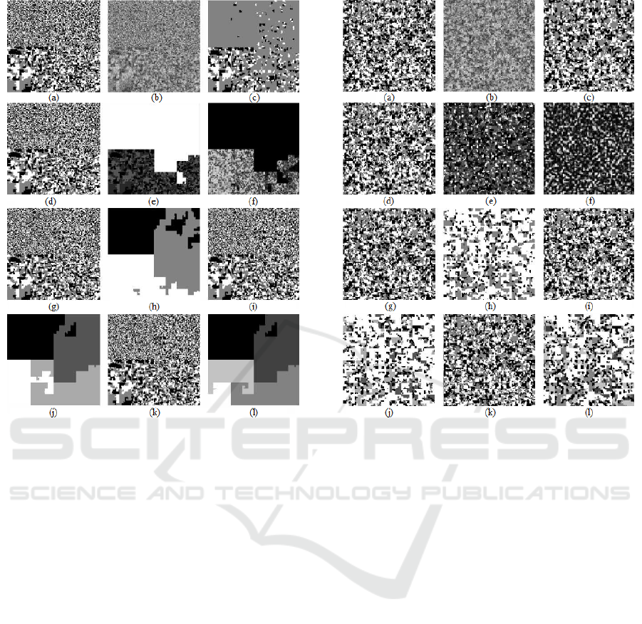
Figure 3: Unsupervised segmentation of sampled nonsta-
tionary data (subset B.3). (a) class-image X = x. (b)
Noised image Y = y. (c) HMC based segmentation, error
ratio τ = 44.5%. (d) HEMC based segmentation, error ratio
τ = 17.4%. (e) HEMC based estimate of U. (f) conditional
weakening coefficient α = 1 −
∑
K
k=1
p(x
n
= ω
k
|y). (g)
SHMC (M=3) based segmentation, error ratio τ = 16.8%.
(h) SHMC (M=3) based estimate of U . (i) SHMC (M=4)
based segmentation, error ratio τ = 16.7%. (j) SHMC
(M=4) based estimate of U . (k) SHMC (M=5) based seg-
mentation, error ratio τ = 16.5%. (l) SHMC (M=5) based
estimate of U.
and hence, SHMC performs relatively bad.
Still, the HEMC makes it possible to handle this
kind of data thanks to its weakening mechanism. In-
deed, notice that the smaller is the value of param-
eter δ
n
, the more intense is the weakening and vice
versa as shown in Fig. 2.g and Fig. 2.h in which
a zoom on the first 1024 values of the parameter
δ
n
and the associated conditional weakening coeffi-
cient α
n
= 1 −
∑
K
k=1
p(x
n
= ω
k
|y) respectively are
depicted. This is due to the fact that for low values
of parameter δ
n
, the observation information is more
important than the prior information, and hence, the
weakening is intense in such sites.
Figure 4: Unsupervised segmentation of sampled nonsta-
tionary data (subset B.4). (a) class-image X = x. (b)
Noised image Y = y. (c) HMC based segmentation, error
ratio τ = 17.5%. (d) HEMC based segmentation, error ratio
τ = 12%. (e) HEMC based estimate of U . (f) conditional
weakening coefficient α = 1 −
∑
K
k=1
p(x
n
= ω
k
|y). (g)
SHMC (M=3) based segmentation, error ratio τ = 12.3%.
(h) SHMC (M=3) based estimate of U . (i) SHMC (M=4)
based segmentation, error ratio τ = 12.3%. (j) SHMC
(M=4) based estimate of U . (k) SHMC (M=5) based seg-
mentation, error ratio τ = 12.2%. (l) SHMC (M=5) based
estimate of U.
3.3 Unsupervised Segmentation of
Binary Class-images Corrupted by
Gaussian White Noise
Let us consider the nonstationary class-images
“Nazca” (sets C.1 and C.2, Fig. 5) and “Zebra” (sets
C.3 and C.4, Fig. 6), of size 128 × 128 and 256 ×
256 respectively. Let Z = (X, Y ) be a nonstation-
ary HMC with Z = (Z
n
)
N
n=1
. Images are converted
to 1D-sequences via Hilbert-Peano scan as done by
(Derrode and Pieczynski, 2004). We then have a re-
alization x with Ω = {ω
1
,ω
2
} where ω
1
and ω
2
cor-
responds to black pixels and white ones respectively.
For sets C.1 and C.3 (resp. sets C.2 and C.4), noisy
images are obtained by drawings from the Gaussian
noise densities N (0, 1) and N (2, 1) (resp. N (0,1)
Unsupervised Segmentation of Nonstationary Data using Triplet Markov Chains
411

Figure 5: Unsupervised segmentation of “Zebra” image. (a)
class-image X = x. (b) Noised image Y = y. (c) HMC
based segmentation, error ratio τ = 6%. (d) HEMC based
segmentation, error ratio τ = 3.6%. (e) HEMC based es-
timate of U . (f) SHMC (M=2) based segmentation, error
ratio τ = 3.7%. (g) HEMC (M=2) based estimate of U . (h)
SHMC (M=3) based segmentation, error ratio τ = 3.3%. (i)
HEMC (M=3) based estimate of U.
and N (1, 1)) associated to ω
1
and ω
2
respectively.
Some obtained segmentation results are illustrated
in Figures 5 and 6. On the other hand, average error
ratios are provided in Table 1 (Subsets C.1–C.2). The
interest of this series of experiments relies in the fact
that the realization of the hidden process is no longer
sampled.
Models provide comparable results with a slight
supremacy of SHMC, which is may be due to the
possibility of partitioning each image into homoge-
Table 1: Average error ratios (%) of unsupervised segmen-
tation of nonstationary data.
Set K-means HEMC
SHMC
M=1 M=2 M=3 M=4 M=5
A 15.5 10.2 15.8 11.4 5.9 5.9 6
B.1 26.1 11.4 25.5 11 10.5 10.4 10.3
B.2 16 12 12.7 12.1 12.1 12 12
B.3 21.7 17.6 45.1 17.8 16.7 16.5 16.5
B.4 21.2 12 17.6 12.2 12.2 12.3 12.2
C.1 27 5 13.3 5.2 4.9 5.2 4.8
C.2 38.7 11 15.4 16.4 14.6 14.1 14.9
C.3 26.1 3.7 6 3.7 3.3 3.3 3.3
C.4 38.5 8.2 12.3 8.1 7.7 7.6 7.7
Figure 6: Unsupervised segmentation of “Nazca” image.
(a) class-image X = x. (b) Noised image Y = y. (c) HMC
based segmentation, error ratio τ = 13.2%. (d) HEMC
based segmentation, error ratio τ = 4.9%. (e) HEMC based
estimate of U. (f) SHMC (M=3) based segmentation, error
ratio τ = 4.9%. (g) HEMC (M=3) based estimate of U . (h)
SHMC (M=7) based segmentation, error ratio τ = 4.7%. (i)
HEMC (M=7) based estimate of U.
neous regions. HEMC assigns the image regions hav-
ing a lot of details to the compound auxiliary class
{ω
1
,ω
1
} to reduce the regularization in such regions.
On the other hand, given a value of M , the SHMC
classifies the image into M “auxiliary” classes shar-
ing similar properties; the regularization within each
auxiliary class is similar to the HMC one.
3.4 Discussion
For all datasets, SHMC and EHMC always provide
better results than conventional HMC. On the other
hand, the supremacy of both models over the blind K-
means clustering shows the interest of considering the
prior information, even when fluctuating, in the seg-
mentation process. Overall, the performances of S-
HMC and HEMC are comparable. The supremacy of
one model over another depends on the kind of data.
4 CONCLUSIONS
In this study, we specified how TMCs can be used
to handle nonstationary data. For this purpose, we
ICEIS 2017 - 19th International Conference on Enterprise Information Systems
412

have considered both Bayesian TMCs (SHMCs) and
evidential ones (SHMCs) with application to unsu-
pervised image segmentation. Performance evalua-
tion of both models with respect to classical HMCs
has been achieved in terms of overall error ratios. It
turned out that both models outperform conventional
HMCs. Furthermore, the evidential model seems a
good solution where no information is available about
the number of stationarities; thanks to the weakening
mechanism that overcomes the lack of precision of
the prior knowledge by searching at each site a good
tradeoff between the a priori and observation infor-
mation. The Bayesian SHMC, on the other hand, is
better-suited when the number of “stationarities” is
known in advance. An interesting extension would
be to tackle the model selection problem to determine
the best-suited model (model choice, number of sta-
tionarities,...) for a given set of data using some crite-
ria such as the Bayesian information criterion (BIC)
as done in (Lanchantin et al., 2011). Another fu-
ture direction would be to combine evidential and
Bayesian models as done in Markov field context for
SAR image segmentation in (Boudaren et al., 2016b;
Boudaren et al., 2016a).
REFERENCES
Ait-El-Fquih, B. and Desbouvries, F. (2005). Bayesian
smoothing algorithms in pairwise and triplet markov
chains. In Statistical Signal Processing, 2005
IEEE/SP 13th Workshop on, pages 721–726. IEEE.
Ait-El-Fquih, B. and Desbouvries, F. (2006). Kalman filter-
ing in triplet Markov chains. Signal Processing, IEEE
Transactions on, 54(8):2957–2963.
An, L., Li, M., Boudaren, M. E. Y., and Pieczynski,
W. (2016). Evidential correlated gaussian mixture
markov model for pixel labeling problem. In Inter-
national Conference on Belief Functions, pages 203–
211. Springer.
Bardel, N. and Desbouvries, F. (2012). Exact Bayesian
prediction in a class of Markov-switching models.
Methodology and Computing in Applied probability,
14(1):125–134.
Baum, L. E., Petrie, T., Soules, G., and Weiss, N. (1970).
A maximization technique occurring in the statistical
analysis of probabilistic functions of Markov chains.
The annals of mathematical statistics, pages 164–171.
Benboudjema, D. and Pieczynski, W. (2007). Unsuper-
vised statistical segmentation of nonstationary im-
ages using triplet Markov fields. Pattern Analy-
sis and Machine Intelligence, IEEE Transactions on,
29(8):1367–1378.
Blanchet, J. and Forbes, F. (2008). Triplet Markov fields
for the classification of complex structure data. Pat-
tern Analysis and Machine Intelligence, IEEE Trans-
actions on, 30(6):1055–1067.
Boudaren, M. E. Y., An, L., and Pieczynski, W.
(2016a). Dempster-Shafer fusion of evidential pair-
wise Markov fields. Approximate Reasoning, Interna-
tional Journal of, 74:13–29.
Boudaren, M. E. Y., An, L., and Pieczynski, W.
(2016b). Unsupervised segmentation of SAR images
using Gaussian mixture-hidden evidential Markov
fields. IEEE Geoscience and Remote Sensing Letters,
13(12):1865–1869.
Boudaren, M. E. Y., Monfrini, E., and Pieczynski, W.
(2011). Unsupervised segmentation of switching pair-
wise Markov chains. In Image and Signal Processing
and Analysis (ISPA), 2011 7th International Sympo-
sium on, pages 183–188. IEEE.
Boudaren, M. E. Y., Monfrini, E., and Pieczynski, W.
(2012a). Unsupervised segmentation of nonstation-
ary pairwise Markov chains using evidential priors. In
EUSIPCO, pages 2243–2247, Bucharest. IEEE.
Boudaren, M. E. Y., Monfrini, E., and Pieczynski, W.
(2012b). Unsupervised segmentation of random dis-
crete data hidden with switching noise distributions.
IEEE Signal Process. Lett., 19(10):619–622.
Boudaren, M. E. Y., Monfrini, E., Pieczynski, W., and
A
¨
ıssani, A. (2012c). Dempster-Shafer fusion of mul-
tisensor signals in nonstationary Markovian context.
EURASIP J. Adv. Sig. Proc., 2012:134.
Boudaren, M. E. Y., Monfrini, E., Pieczynski, W., and Ais-
sani, A. (2014). Phasic triplet Markov chains. IEEE
Transactions on Pattern Analysis and Machine Intel-
ligence, 36(11):2310–2316.
Boudaren, M. E. Y. and Pieczynski, W. (2016a). Dempster-
Shafer fusion of evidential pairwise Markov chains.
Fuzzy Systems, IEEE Transactions on, 24(6):1598–
1610.
Boudaren, M. E. Y. and Pieczynski, W. (2016b). Unified
representation of sets of heterogeneous Markov tran-
sition matrices. Fuzzy Systems, IEEE Transactions on,
24(2):497–503.
Bricq, S., Collet, C., and Armspach, J.-P. (2006). Triplet
Markov chain for 3D MRI brain segmentation using a
probabilistic atlas. In Biomedical Imaging: Nano to
Macro, 2006. 3rd IEEE International Symposium on,
pages 386–389. IEEE.
Capp
´
e, O., Moulines, E., and Ryd
´
en, T. (2005). Inference
in hidden Markov models, volume 6. Springer, New
York.
Celeux, G., Chauveau, D., and Diebolt, J. (1996). Stochas-
tic versions of the EM algorithm: an experimental
study in the mixture case. Journal of Statistical Com-
putation and Simulation, 55(4):287–314.
Dehghani, H., Vahidi, B., Naghizadeh, R., and Hosseinian,
S. (2013). Power quality disturbance classification
using a statistical and wavelet-based hidden Markov
model with Dempster–Shafer algorithm. Interna-
tional Journal of Electrical Power & Energy Systems,
47:368–377.
Delmas, J. P. (1997). An equivalence of the EM and ICE
algorithm for exponential family. IEEE transactions
on signal processing, 45(10):2613–2615.
Unsupervised Segmentation of Nonstationary Data using Triplet Markov Chains
413

Derrode, S. and Pieczynski, W. (2004). Signal and image
segmentation using pairwise Markov chains. Signal
Processing, IEEE Transactions on, 52(9):2477–2489.
Forney Jr, G. D. (1973). The Viterbi algorithm. Proceedings
of the IEEE, 61(3):268–278.
Foucher, S., Germain, M., Boucher, J.-M., and Benie, G. B.
(2002). Multisource classification using ICM and
Dempster-Shafer theory. IEEE Transactions on In-
strumentation and Measurement, 51(2):277–281.
Fouque, L., Appriou, A., and Pieczynski, W. (2000). An
evidential Markovian model for data fusion and unsu-
pervised image classification. In Information Fusion,
2000. FUSION 2000. Proceedings of the Third Inter-
national Conference on, volume 1, pages TUB4–25.
IEEE.
Gan, L., Wu, Y., Liu, M., Zhang, P., Ji, H., and Wang,
F. (2012). Triplet Markov fields with edge location
for fast unsupervised multi-class segmentation of syn-
thetic aperture radar images. IET image processing,
6(7):831–838.
Habbouchi, A., Boudaren, M. E. Y., A
¨
ıssani, A., and
Pieczynski, W. (2016). Unsupervised segmentation
of markov random fields corrupted by nonstationary
noise. IEEE Signal Processing Letters, 23(11):1607–
1611.
Lanchantin, P., Lapuyade-Lahorgue, J., and Pieczynski,
W. (2011). Unsupervised segmentation of randomly
switching data hidden with non-Gaussian correlated
noise. Signal Processing, 91(2):163–175.
Lanchantin, P. and Pieczynski, W. (2005). Unsupervised
restoration of hidden nonstationary Markov chains us-
ing evidential priors. Signal Processing, IEEE Trans-
actions on, 53(8):3091–3098.
Lapuyade-Lahorgue, J. and Pieczynski, W. (2006). Un-
supervised segmentation of hidden semi-Markov non
stationary chains. In Bayesian Inference and Max-
imum Entropy Methods in Science and Engineer-
ing(AIP Conference Proceedings Volume 872), vol-
ume 872, pages 347–354. Citeseer.
Le H
´
egarat-Mascle, S., Bloch, I., and Vidal-Madjar, D.
(1998). Introduction of neighborhood information in
evidence theory and application to data fusion of radar
and optical images with partial cloud cover. Pattern
recognition, 31(11):1811–1823.
Liu, G., Li, M., Wu, Y., Zhang, P., Jia, L., and Liu, H.
(2014). Polsar image classification based on wishart
TMF with specific auxiliary field. Geoscience and Re-
mote Sensing Letters, IEEE, 11(7):1230–1234.
McLachlan, G. and Krishnan, T. (2007). The EM algorithm
and extensions, volume 382. John Wiley & Sons, New
Jersey.
Park, J., Chebbah, M., Jendoubi, S., and Martin, A. (2014).
Second-order belief hidden markov models. In Belief
Functions: Theory and Applications, pages 284–293.
Springer.
Pieczynski, W. (2003). Pairwise Markov chains. Pat-
tern Analysis and Machine Intelligence, IEEE Trans-
actions on, 25(5):634–639.
Pieczynski, W. (2007). Multisensor triplet Markov chains
and theory of evidence. International Journal of Ap-
proximate Reasoning, 45(1):1–16.
Pieczynski, W. and Benboudjema, D. (2006). Multisensor
triplet Markov fields and theory of evidence. Image
and Vision Computing, 24(1):61–69.
Pieczynski, W., Hulard, C., and Veit, T. (2003). Triplet
Markov chains in hidden signal restoration. In Inter-
national Symposium on Remote Sensing, pages 58–68.
International Society for Optics and Photonics.
Rabiner, L. (1989). A tutorial on hidden Markov models
and selected applications in speech recognition. Pro-
ceedings of the IEEE, 77(2):257–286.
Ramasso, E. (2009). Contribution of belief functions to
hidden Markov models with an application to fault
diagnosis. In Proceedings of the IEEE International
Workshop on Machine Learning for Signal Process-
ing., pages 1–6.
Reineking, T. (2011). Particle filtering in the Dempster–
Shafer theory. International Journal of Approximate
Reasoning, 52(8):1124–1135.
Shafer, G. (1976). A mathematical theory of evidence, vol-
ume 1. Princeton university press Princeton, Prince-
ton.
Soubaras, H. (2010). On evidential Markov chains. In Foun-
dations of reasoning under uncertainty, pages 247–
264. Springer, Berlin Heidelberg.
Tupin, F., Bloch, I., and Ma
ˆ
ıtre, H. (1999). A first step
toward automatic interpretation of SAR images using
evidential fusion of several structure detectors. Geo-
science and Remote Sensing, IEEE Transactions on,
37(3):1327–1343.
Wang, F., Wu, Y., Zhang, Q., Zhang, P., Li, M., and Lu,
Y. (2013). Unsupervised change detection on SAR
images using triplet Markov field model. Geoscience
and Remote Sensing Letters, IEEE, 10(4):697–701.
Wu, Y., Zhang, P., Li, M., Zhang, Q., Wang, F., and
Jia, L. (2013). SAR image multiclass segmentation
using a multiscale and multidirection triplet markov
fields model in nonsubsampled contourlet transform
domain. Information Fusion, 14(4):441–449.
Yoji, Y., Tetsuya, M., Yoji, U., and Yukitaka, S. (2003).
A method for preventing accidents due to human ac-
tion slip utilizing HMM-based Dempster-Shafer the-
ory. In Robotics and Automation, 2003. Proceed-
ings. ICRA’03. IEEE International Conference on,
volume 1, pages 1490–1496. IEEE.
Zhang, P., Li, M., Wu, Y., Gan, L., Liu, M., Wang, F., and
Liu, G. (2012a). Unsupervised multi-class segmenta-
tion of SAR images using fuzzy triplet Markov fields
model. Pattern Recognition, 45(11):4018–4033.
Zhang, P., Li, M., Wu, Y., Liu, M., Wang, F., and
Gan, L. (2012b). SAR image multiclass segmenta-
tion using a multiscale TMF model in wavelet do-
main. Geoscience and Remote Sensing Letters, IEEE,
9(6):1099–1103.
ICEIS 2017 - 19th International Conference on Enterprise Information Systems
414
