
Robust Statistical Prior Knowledge for Active Contours
Prior Knowledge for Active Contours
Mohamed Amine Mezghich, Ines Sakly, Slim Mhiri and Faouzi Ghorbel
GRIFT Research Group, CRISTAL Laboratory,
National School of Computer Science, University of Manouba, La Manouba 2010, Tunisie
{amine.mezghich, slim.mhiri, ines.sakly, faouzi.ghorbel}@ensi-uma.tn
Keywords:
Active Contours, Prior Knowledge, Shape Descriptors, Linear Discriminant Analysis, Estimation-
Maximization.
Abstract:
We propose in this paper a new method of active contours with statistical shape prior. The presented approach
is able to manage situations where the prior knowledge on shape is unknown in advance and we have to
construct it from the available training data. Given a set of several shape clusters, we use a set of complete,
stable and invariants shape descriptors to represent shape. A Linear Discriminant Analysis (LDA), based on
Patrick-Fischer criterion, is then applied to form a distinct clusters in a low dimensional feature subspace. Fea-
ture distribution is estimated using an Estimation-Maximization (EM) algorithm. Having a currently detected
front, a Bayesian classifier is used to assign it to the most probable shape cluster. Prior knowledge is then con-
structed based on it’s statistical properties. The shape prior is then incorporated into a level set based active
contours to have satisfactory segmentation results in presence of partial occlusion, low contrast and noise.
1 INTRODUCTION
Active contour methods have been introduced in 1988
(M. Kass and Terzopolous, 1988). The principle con-
sists in moving a curve iteratively minimizing energy
functional. The minimum is reached at object bound-
aries. Active contour methods can be classified into
two families: parametric and geometric active con-
tours. The first family, called also snakes, uses an
explicit representation of the contours and depends
only on image gradient to detect objects. The second
one uses an implicit representation of the contours by
level set approach to handle topological changes of
the front. A number of active contour models based
on level set theory have been then proposed which
can be divided into two categories : The boundary-
based approach which depends on an edge stopping
function to detect objects (Malladi and Vemuri, 1995;
V. Caselles and Sapiro, 1997) and the region-based
approach which is based on minimizing an energy
functionnal to segment objects in the image (T.F.Chan
and L.A.Vese, 2001). Experiments show that region-
based models can detect objects with smooth bound-
aries and noise since the whole region is explored.
However, there is still no way to characterize the
global shape of an object. Especially in presence of
occlusions and clutter, all the previous models con-
verge to the wrong contours.
To solve the above mentioned problems, different
attempts include shape prior information into the ac-
tive contour models. Many works have been proposed
which can be classified into statistical or geometric
shape prior. (M. Leventon and Faugeras, 2000), as-
sociated a statistical shape model to the geodesic ac-
tive contours (V. Caselles and Sapiro, 1997). A set
of training shapes is used to define a Gaussian distri-
bution over shapes. At each step of the surface evo-
lution, the maximum a posteriori position and shape
are estimated and used to move globally the surface
while local evolution is based on image gradient and
curvature. (Chen and Geiser, 2001) defined an en-
ergy functional based on the quadratic distance be-
tween the evolving curve and the average shapes of
the target object after alignment. This term is then
incorporated into the geodesic active contours.
(Fang and Chan, 2007) introduced a statistical
shape prior into geodesic active contour to detect par-
tially occluded object. PCA is computed on level set
functions used as training data and the set of points in
subspace is approximated by a Gaussian function to
construct the shape prior model. To speed up the algo-
rithm, an explicit alignment of shape prior model and
the current evolving curve is done to calculate pose
parameters unlike (M. Leventon and Faugeras, 2000)
where a MAP of pose is performed.
(M.A. Charmi and Ghorbel, 2008) introduced a
Mezghich M., Sakly I., Mhiri S. and Ghorbel F.
Robust Statistical Prior Knowledge for Active Contours - Prior Knowledge for Active Contours.
DOI: 10.5220/0006268306450650
In Proceedings of the 12th International Joint Conference on Computer Vision, Imaging and Computer Graphics Theory and Applications (VISIGRAPP 2017), pages 645-650
ISBN: 978-989-758-225-7
Copyright
c
2017 by SCITEPRESS – Science and Technology Publications, Lda. All rights reserved
645

new geometric shape prior into the snake model. A
set of complete and locally stable invariants to Eu-
clidean transformations (Ghorbel, 1998) is used to de-
fine new force which makes the snake overcome some
well-known problems. In (M-A. Mezghich, 2013),
a new geometric shape prior for a region-based ac-
tive contour (T.F.Chan and L.A.Vese, 2001) was de-
fined which is based on shape registration by phase
correlation using Fourier Transform. The method
presented encouraging segmentation results in pres-
ence of partial occlusion, cluder and noise under rigid
transformation. Similar work was presented in (M-
A. Mezghich and F.Ghorbel, 2014) for an edge based
active contours (Malladi and Vemuri, 1995) to help
the curve reach the true contours of the object of in-
terest.
For all the above presented approaches, the shape
or the model of reference is known in advance. To
generalize the idea of shape prior to more complex
situations where many models of reference are avail-
able and we have to choose to most suitable one, some
works have been presented.
In (Fang and Chan, 2006) a statistical shape prior
model is presented to give more robustness to object
detection. This shape prior is able to manage differ-
ent states of the same object, thus a Gaussian Mixture
Model (GMM) and a Bayesian classifier framework
are used. Using the level set functions for represent-
ing shape, this model suffer from the curse of dimen-
sionality. Hence PCA was used to perform dimen-
sionality reduction.
In (A.Foulonneau and Heitz, 2009) a multi-
references shape prior is presented for a region-based
active contours. Prior knowledge is defined as a dis-
tance between shape descriptors based on the Legen-
dre moments of the characteristic function of many
available shapes.
In this paper, we focus on extending the work
presented in (I. Sakly and F.Ghorbel, 2016) that
construct a statistical shape prior from a given single
cluster of similar shapes according to the object to
be detected. Inspired from the paper of (Tsai A,
2005), in which the EM algorithm was used for shape
classification into different clusters based on level set
representation, we propose to represent the available
training data by an invariant set of complete shape
descriptors. Then a dimensionality reduction will be
performed based on LDA to have a separated shape
clusters that respect to Patrick-Fischer criterion.
For each cluster, we computed a statistical map to
be used as shape prior. In the reduced subspace,
the EM algorithm will be applied to estimated data
distribution. For the current evolving curve, we
use a Bayesian classifier to assign it to the most
probable cluster. The improved model can retain all
the advantages of level set based model and have the
additional ability of being able to handle the case
of multi-reference shape knowledge in presence of
partial occlusions.
The remainder of this paper is organized as fol-
lows : In Section 2, we recall the principle of level set
based active contour models. Then, the construction
of a multi-reference shape prior constraint will be pre-
sented in Section 3. The incorporation of shape prior
and the evolving schema will be presented in Section
4. Some experimental results are presented in Section
5. Finally, we conclude the work and highlight some
possible perspectives in Section 6.
2 LEVEL SET BASED ACTIVE
CONTOURS
The basic idea of the Level Set approach (Malladi and
Vemuri, 1995) is to consider the initial contour as the
zero level set of a higher dimension function called
level set function and following the evolution of this
embedding function, we deduce the contour evolution
by seeking its zero level set at each iteration. Several
models have been proposed in literature that we can
classify into edge-based or region-based active con-
tours. In (Malladi and Vemuri, 1995), the authors pro-
posed the basic level set model which is based on an
edge stopping function g. The evolutions equation of
the level set function φ is
φ
n+1
(x,y) = φ
n
(x,y) + ∆tg(x, y)F(x,y)|∇φ
n
(x,y)|,
(1)
F is a speed function of the form F = F
0
+ F
1
(K)
where F
0
is a constant advection term equals to (±1)
depends of the object inside or outside the initial con-
tour. The second term is of the form −εK where K is
the curvature at any point and ε > 0.
g(x,y) =
1
1+|∇G
σ
∗ f (x,y)|
,
(2)
where f is the image and G
σ
is a Gaussian filter with
a deviation equals to σ. This stopping function has
values that are closer to zero in regions of high image
gradient and values that are closer to unity in regions
with relatively constant intensity.
It’s obvious that for this model, the evolution is
based on the image gradient. That’s why, this model
leads to unsatisfactory results in presence of occlu-
sions, low contrast and even noise.
VISAPP 2017 - International Conference on Computer Vision Theory and Applications
646

3 SHAPE PRIOR FORMULATION
We will devote this section to present our multi-
refrences shape prior constraint to be added to a level
set based active contours. Our algorithm is composed
of two steps:
1− An off-line step which consists in represent-
ing the training data by an invariants set of shape
descriptors instead of using level set to avoid data
alignment which is a hard task to perform for all the
data. Then, the estimation of data distribution over
different clusters in a reduced subspace using the EM
algorithm after performing the LDA method.
2− An on-line step which consists in assigning the
evolving front to the most probable cluster based on a
Bayesian classifier.
3.1 Shape Description using Invariant
Descriptors
Given a training data, we perform a level set segmen-
tation of each object to determine the curve that rep-
resents the shape of the object of interest. Then we
compute an invariants set of shape description intro-
duced in (Ghorbel, 1998) as follows:
I
k
0
(γ) = |C
k
0
(γ)|, C
k
0
(γ) 6= 0
I
k
1
(γ) = |C
k
1
(γ)|, C
k
1
(γ) 6= 0, k
1
6= k
0
I
k
(γ) =
C
k
(γ)
k
0
−k
1
C
k
0
(γ)
k−k
1
C
k
1
(γ)
k
0
−k
I
k−k
1
−p
k
0
(γ)I
k
0
−k−q
k
1
(γ)
,k 6= k
0
,k
1
;
p,q > 0,
This set is complete, stable and invariant to rigid
transformations.The stability criterion expresses the
fact that a small distortion of the shape does not in-
duce a noticeable divergence. This property makes
invariant descriptors robust under small shape varia-
tions. To compare shapes, we used the following dis-
tance:
d(γ
1
,γ
2
) =
∑
k
(|I
k
(γ
1
) − I
k
(γ
2
)|
1
2
)
2
(3)
After this step, we obtain an invariants representation
of the training data.
3.2 Dimensionality Reduction using
Linear Discriminant Analysis
The second step of our approach consists on perform-
ing dimensionality reduction of data represented by
the previous invariants features. We were based on the
Fisher Linear Discriminant Analysis (FLDA). This
method intends to reduce the dimension, so that in
the new space, the between class distances are max-
imized while the within class distances are minimiz-
ing. To that purpose, FLDA considers searching for
orthogonal linear projection matrix w that maximizes
the following so called Fischer optimization criterion
see (Fukunaga, 1990) and (Ghorbel and la Tocnaye,
1990):
J(w) =
tr(w
T
S
b
w)
tr(w
T
S
w
w)
(4)
S
w
is the within class scatter matrix and S
b
is the be-
tween class scatter one. They are given by
S
w
=
c
∑
k=1
π
k
E
k
[(X − µ
k
)(X − µ
k
)
T
]
(5)
S
b
=
c
∑
k=1
π
k
(µ
k
− µ)(µ
k
− µ)
T
(6)
where µ
k
=E
k
[X] is the conditional expectation of
the multidimensional random vector X given the class
k, µ corresponds to the mean vector over all classes
and π
k
denote the prior probability of the k
th
class.
Because its not practical to find an analytical solu-
tion w that verify the J criteria, one possible subopti-
mal solution is to choose w formed by the d first eigen
vectors of S
−1
w
S
b
those correspond to the d largest
eigen values. After computation of w, the FLDA
method proceeds to the projection of the original data
into the reduced space spanned by the vectors of w un-
like the work of (Fang and Chan, 2006), where Princi-
pal Component Analysis (PCA) was used to perform
data projection.
3.3 The EM Algorithm for Data
Distribution Estimation
The EM algorithm proposed by (Dempster, 1977) is
a powerful iterative technique suited for calculating
the maximum-likelihood (ML) estimates in problems
where parts of the data are missing. The missing
data in our EM formulation is the class labels K. If
the class labels for the different shapes within the
database are known, then we can determine for which
cluster belongs the current evolving contour. The
method opts for estimating the probability densities
of any mixture by a usual law while approaching as
closely as possible the actual distribution of the ini-
tial mixture. In other words, the EM algorithm opts to
maximize the likelihood between the probability den-
sity and the histogram of the initial mixture.
The observed data in our EM formulation is X that
corresponds to the collection of data obtained after
FLDA reduction. Finally, Y is the class label of each
Robust Statistical Prior Knowledge for Active Contours - Prior Knowledge for Active Contours
647

feature to be estimated in our formulation. Let:
π
k
= P[Y = k] the prior probability,
π
x
k
= P[Y = k/X = x] the posterior probability,
f
k
(x) = P[X = x/Y = k] the conditional probability,
f
X
(x) =
∑
K
k=1
f
k
(x).
After estimating the value of π
k
and f
k
using the EM
algorithm, we can deduce the class of each element
based on Bayes rule :
K(x) = arg(max
k
(π
x
k
)) = arg(max
k
(π
k
f
k
(x)))
(7)
4 ACTIVE CONTOURS WITH
SHAPE PRIOR
In (M-A. Mezghich and F.Ghorbel, 2014) a new way
to introduce shape prior to the presented level set
model in section 2. The idea is to define a new stop-
ping function that update the evolving level set func-
tion in the region of variability between the active
contour and the reference until convergence is ob-
tained.
g
shape
(x,y) =
0, i f φ
prod
(x,y) >= 0,
sign(φ
re f
(x,y)),else,
(8)
where φ
prod
(x,y) = φ(x, y) · φ
re f
(x,y), φ is the level
set function associated to the evolving contour, while
φ
re f
is the level set function associated to the shape of
reference after alignment. As it can be seen, the new
proposed stopping function only allows for updating
the level set function in the regions of variability be-
tween shapes. In these regions g
shape
is either 1 or
-1 because in the case of partial occlusions, the func-
tion is equals to 1 in order to push the edge inward
(deflate) and in case of missing parts, this function is
equals to -1 to push the contour towards the outside
(inflate). In our work, the direction of evolution is
handled automatically based on the sign of φ
re f
. The
total discrete evolution’s equation that we propose is
as follows
φ
n+1
(i, j)−φ
n
(i, j)
∆t
=
((1 − w) g(i, j) + w g
shape
(i, j))F(i, j)|∇φ
n
(i, j)|,
(9)
w is a constant weighting factor between the image-
based force and knowledge-driven force, generally
chosen > 0.5 to promote the evolution towards the
reference shape.
We generalized the approach in the recent work
(I. Sakly and F.Ghorbel, 2016) for the case of several
references of the same shape. In fact, in some fields
like in medical context, generally the prior informa-
tion on shape is obtained from a training data. For
this reason, we propose a dynamic weighting term
w which takes into account the statistical properties
of the given cluster of shapes. Hence, the evolving
contour will converge to the most probable front.
For each pixel x(i, j) of the image, we will count
its degree of belonging to the target object, i.e. the
number of times over all the training set, the pixel be-
longs to the target shape. Then we will name it w(i, j).
Hence, to incorporate a prior knowledge based on
a set of similar shapes, the proposed model is:
φ
n+1
(i, j)−φ
n
(i, j)
∆t
=
((1 − w(i, j)) g(i, j) + w(i, j) g
shape
(i, j))F(i, j)|∇φ
n
(i, j)|,
(10)
5 EXPERIMENTAL RESULTS
We will start this section by describing our algorithm,
then we will comment the obtained results on simu-
lated and real data.
5.1 The Approach’s Algorithm
The proposed approach is composed of two steps as
follows:
Algorithm 1 : Multi-references shape prior for active con-
tour.
1: Off-Line step
2: For each cluster C
k
of similar shapes (represented
by level set function φ), we compute it’s statistical
map w
k
.
3: We compute the invariants set of shape descrip-
tors for all the training data as presented in sec-
tion 3.1.
4: We perform the FLDA method on the obtained
invariants description of shapes.
5: We estimate the data distribution over different
clusters in a reduced subspace using the EM al-
gorithm.
6: On-Line step
7: Apply the classic level set based active contour
until the evolving contour became stable (equa-
tion 1).
8: Assign the detected front to the most similar clus-
ter C
k
based on Bayes classifier (equation 7).
9: Continue the evolution based on both the statisti-
cal map w
k
of the selected cluster that represent
the shape prior and the image data represented by
the gradient(equation 10).
VISAPP 2017 - International Conference on Computer Vision Theory and Applications
648
5.2 Application to Simulated Data
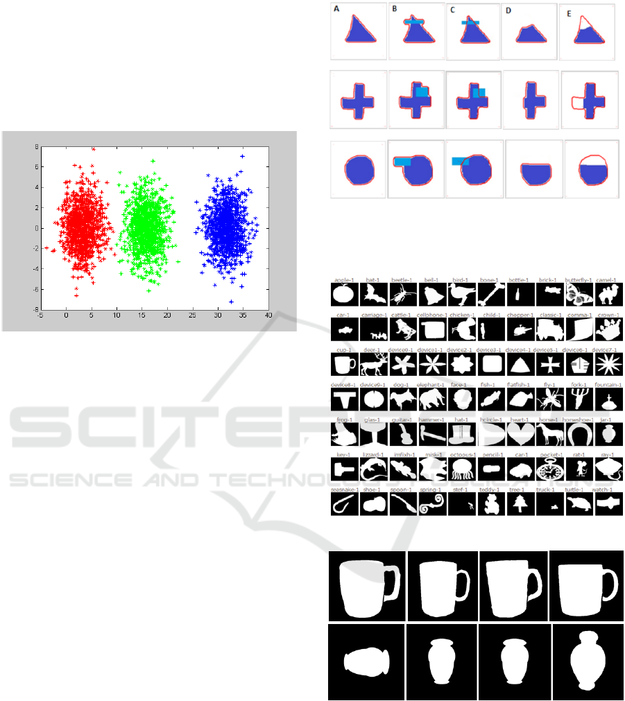
We consider a mixture of 3 clusters generated by
a multivariate normal distribution N
k
(µ
k
,σ
k
); k ∈
{1,2,3} . Each cluster C
k
is composed of 1000 items
and each item has 10 dimensions. The figure below
shows data distribution in the reduced space formed
by the two largest eigenvectors.
Figure 1: Data distribution in the reduced features space.
As it can be seen, the clusters are well separated
in the reduced subspace. Performing an EM classifi-
cation of this data, we obtain 1 misclassified element
from the available 3000 items. The errors is about
1/3000
5.3 Application to the Segmentation
Problem
For the experiment below, we consider 3 different
clusters of shapes (triangle, plus and circle). Given
that the invariant descriptors presented in section 3.1
are complex numbers, i.e each descriptor I
k
= r
k
e
iθ
k
,
we assign for each shape a characteristic vector U =
[r
1
..r
n
θ
1
..θn]
T
. The FLDA will be applied on the N
characteristic vectors U.
In fig.2, the first, second and fourth columns
represent the segmentation result without prior in-
formation. The third and last ones represent the
segmentation result using the proposed approach.
This result improves the robustness of the segmen-
tation process in presence of missing parts and par-
tial occlusions of the target objects. Similar ex-
periment was performed on the MPEG − 7 shape
data base (link : http://www.cis.temple.edu/ late-
cki/TestData/mpeg7shapeB.tar.gz). Some shapes of
this data base are presented in fig.3.
We consider two classes of shapes fig.4. For each
class, we take 20 examples for learning. The descrip-
tors distribution according to the first two axes ares
presented in fig.5.
Figure 2: Comparison of the segmentation results of
(A,B,D) traditional active contour without using shape prior
model and (C,E) our proposed method using shape prior
model for partially occluded objects.
Figure 3: A selected set of MPEG7 data base.
Figure 4: A selected two shape classes (a Cup and a Jar).
Segmentation results with the proposed model are
show in fig.6.
6 CONCLUSIONS
A novel method of level set based active contours with
statistical shape prior is presented in this paper. An in-
Robust Statistical Prior Knowledge for Active Contours - Prior Knowledge for Active Contours
649

Figure 5: Features distribution in the reduced subspace.
Figure 6: Segmentation results without shape prior (first
row) and with shape prior (second row).
variant and complete set of shape descriptors is used
to represent the training data. Then a Linear Discrim-
inant Analysis (LDA) is applied to form a separated
shape clusters in a low dimensional feature subspace.
An EM algorithm is then performed to estimate the
data distribution. Given an evolving curve, we com-
pute it’s set of shape descriptors then we assign it to
the most similar cluster based on a Bayesian classifier.
The prior knowledge is obtained from the statistical
map of that cluster. In the subsequent curve evolu-
tion, our model will depends on both data and prior
knowledge to recover the true contour of the object of
interest.
REFERENCES
A.Foulonneau, P. C. and Heitz, F. (2009). Multi-reference
shape priors for active contours. In Int J Comput Vi-
sion, 81, pp.68-81.
Chen, Y., T. S. T. H. H. F. W. D. and Geiser, E. (2001).
On the incorporation of shape priors into geometric
active contours. In In IEEE Workshop on Variational
and Level Set Methods in Computer Vision.
Dempster, A., L. N. R. D. (1977). Maximum-likelihood
from incomplete data via the em algorithm. In J. Royal
Stat. Soc. Ser. B 39, 138.
Fang, W. and Chan, K. (2006). Using statistical shape priors
in geodesic active contours for robust object detection.
In Proceedings of the 18th International Conference
on Pattern Recognition - Volume 02, p.304-307.
Fang, W. and Chan, K. (2007). Incorporating shape
prior into geodesic active contours for detecting
partially occluded object. In Pattern Recognition,
40(8):21632172.
Fukunaga, K. (1990). Introduction to statistical pattern clas-
sification. In Academic Press.
Ghorbel, F. (1998). Towards a unitary formulation for in-
variant image description:application to image cod-
ing. In An. of telecom., vol.153,no.3 pp. 145-155.
Ghorbel, F. and la Tocnaye, J. L. B. (1990). Automatic con-
trol of lamellibranch larva growth using contour in-
variant feature extraction. In Pattern Recognition, vol.
23, no. 3/4, pp. 319-323.
I. Sakly, M-A. Mezghich, S. and F.Ghorbel (2016). A hy-
brid shape constraint for level set-based active con-
tours. In IEEE International Conference on Imaging
Systems and Techniques (IST).
M-A. Mezghich, S. and F.Ghorbel (2014). Invariant shape
prior knowledge for an edge-based active contours. In
VISAPP (2): 454-461.
M-A. Mezghich, M. Sellami, S. M. F. G. (2013). Robust
object segmentation using active contours and shape
prior. In ICPRAM, p.547-553.
M. Kass, A. W. and Terzopolous, D. (1988). Snakes: active
contour models. In Int. J. of Comp.Vis., 1(4):321 331.
M. Leventon, E. G. and Faugeras, O. (2000). Statistical
shape influence in geodesic active contours. In In
Proc. of IEEE Conference on Computer Vision and
Pattern Recognition,p.316323.
M.A. Charmi, S. D. and Ghorbel, F. (2008). Fourier-based
shape prior for snakes. In Pat. Recog. Let., vol.29(7),
pp. 897-904.
Malladi, R., S. J. and Vemuri, B. (1995). Shape modeling
with front propagation: A level set approach. In In
IEEE Trans. Patt. Anal. Mach. Intell, 1995.
T.F.Chan and L.A.Vese (2001). Active contours without
edges. In IEEE Transactions on Image Processing,
10(2):266277.
Tsai A, Wells WM, W. S. W. A. (2005). An em algorithm
for shape classification based on level sets. In Medical
Image Analysis. Vol.9(5), p.491-502.
V. Caselles, R. K. and Sapiro, G. (1997). Geodesic active
contours. In Int. J. of Comp. Vis., 22(1):6179.
VISAPP 2017 - International Conference on Computer Vision Theory and Applications
650
