Pedestrian Counting using Deep Models Trained on Synthetically
Generated Images
Sanjukta Ghosh
1,2
, Peter Amon
2
, Andreas Hutter
2
and Andr´e Kaup
1
1
Multimedia Communications and Signal Processing, Friedrich-Alexander-Universit¨at Erlangen-N¨urnberg (FAU),
Erlangen, Germany
2
Sensing and Industrial Imaging, Siemens Corporate Technology, Munich, Germany
Keywords:
Pedestrian Counting, Deep Learning, Convolutional Neural Networks, Synthetic Images, Transfer Learning,
Cross Entropy Cost Function, Squared Error Cost Function.
Abstract:
Counting pedestrians in surveillance applications is a common scenario. However, it is often challenging to
obtain sufficient annotated training data, especially so for creating models using deep learning which require
a large amount of training data. To address this problem, this paper explores the possibility of training a deep
convolutional neural network (CNN) entirely from synthetically generated images for the purpose of counting
pedestrians. Nuances of transfer learning are exploited to train models from a base model trained for image
classification. A direct approach and a hierarchical approach are used during training to enhance the capability
of the model for counting higher number of pedestrians. The trained models are then tested on natural images
of completely different scenes captured by different acquisition systems not experienced by the model during
training. Furthermore, the effectiveness of the cross entropy cost function and the squared error cost function
are evaluated and analyzed for the scenario where a model is trained entirely using synthetic images. The
performance of the trained model for the test images from the target site can be improved by fine-tuning using
the image of the background of the target site.
1 INTRODUCTION
Deep neural networks (LeCun et al., 2015), (Bengio
and Courville, 2016) have been successfully used for
numerous applications for visual sensor data. The
models generated by training deep neural networks
have been shown to learn useful features for different
tasks like object detection (Girshick et al., 2013),
(Angelova et al., 2015a), (Angelova et al., 2015b),
classification (Krizhevsky et al., 2012) and a lot
of other applications. In surveillance applications,
a common question is to estimate the number of
pedestrians in a certain area. One approach is to
explicitly detect the pedestrians first and then do
the counting. With the ability of deep learning
systems to perform end-to-end learning, it is possible
to train deep neural networks to count the number
of pedestrians in a scene directly. This has been
demonstrated in (Segui et al., 2015) and (Zhang
et al., 2015) for digits, people and crowd counting.
However, in practical applications, there may not be
much or in the extreme case, no labeled training data
available. Moreover, there may not be training data
available for the specific camera to be used or the
scenes of the target site.
To address this challenge, on the one hand
we compose synthetic training images from parts
of natural images and on the other use a CNN
model trained for an image classification task as
the base model to tune for our task of counting
pedestrians. Our approach is to use transfer learning
and synthetically generated images to tune a CNN to
count pedestrians. The pedestrian counting problem
is considered in two ways: as a classification
problem using the cross entropy cost function and
as a regression problem using the squared error cost
function. Both the cases are evaluated for this
scenario where the model is trained completely on
synthetic images and it is required to generalize
well so that meaningful results are obtained for the
target data that have not been experienced at all
by the model during training. Initially, a baseline
model to count a limited number of pedestrians in
a single frame is established. The capability of the
model is then enhanced to count a higher number of
pedestrians in a single frame. The trained models
were tested on natural images of the UCSD dataset
86
Ghosh S., Amon P., Hutter A. and Kaup A.
Pedestrian Counting using Deep Models Trained on Synthetically Generated Images.
DOI: 10.5220/0006132600860097
In Proceedings of the 12th International Joint Conference on Computer Vision, Imaging and Computer Graphics Theory and Applications (VISIGRAPP 2017), pages 86-97
ISBN: 978-989-758-226-4
Copyright
c
 2017 by SCITEPRESS – Science and Technology Publications, Lda. All rights reserved

(Chan et al., 2008) and found to give meaningful
results. By using only the image of the background
of the target data set along with the synthetic images
for fine-tuning the pedestrian counting model, the
performance on the target data set was found to
improve.
The main contributions of this paper are:
1) While the concepts of transfer learning and using
synthetic images are not new individually, the use
of synthetically generated images (Section 3.2) along
with transfer learning for training deep models for
counting pedestrians (Sections 3.3, 4.1 and 4.2) is
a novel approach. Data scarcity and training data
annotation problems are mitigated by using synthetic
images. The advantage of using transfer learning is
that one can generate the models quickly without a
full-fledged lengthy training using large amount of
training data.
2) To enhance the capability of the model, the
rationale of using increasingly complex images for
training is used in place of feeding the network with
all the complexities of the training images at once
(Section 4.2).
3) Analysis and establishing the suitability of the
cross entropy cost function over the squared error
cost function for this scenario where training is
entirely on synthetic images and the model is required
to generalize across scenes and acquisition devices
(Section 4.3).
2 RELATED WORK
2.1 Synthetic Data Generation
Hattori et al. (Hattori et al., 2015) propose a technique
for scene-specific and location-specific pedestrian
detection in the absence of any real training data
for a scene. Synthetic training data is generated by
leveraging the geometric information of the scene to
simulate pedestrian appearance at various locations
considering the static parts of the scene like presence
of walls. In (Ros et al., 2016), synthetic data
is generated for training a CNN for the task of
semantic segmentation of scenes. The SYNTHIA
dataset which is a collection of synthetic images and
videos of urban scenarios with pixel level annotations
is generated. The UNITY development platform
is used to render scenes of a city considering
different scenarios with elements encountered while
driving. Richter et al. (Richter et al., 2016)
use computer games to generate synthetic training
data with annotations for semantic segmentation
of images. This is achieved by intercepting the
communication between the game and the graphics
hardware and analyzing the resource types used to
compose a scene.
2.2 Pedestrian Counting using
Hand-crafted Features
Lemptisky et al. (Lempitsky and Zisserman, 2010)
estimate the image density by training a model based
on a regularized quadratic cost function. The integral
of the density over an area is used to find the count
of pedestrians. Merad et al. (Merad et al., 2010)
count pedestrians from images by using the skeleton
graph process to segment the body and detecting
heads. Fujii et al. (Fujii et al., 2010) first extract
candidate regions and segment into blobs. Features
extracted from each blob are used to train a neural
network which is the used to estimate the count of
pedestrians. Fiaschi et al. (Fiaschi et al., 2012) use
random regression forests to estimate the density of
objects per pixel which are then used for counting
pedestrians. Yu et al. (Yu et al., 2014) count
pedestrians by doing a spatio-temporal analysis of
a sequence of frames. In (Arteta et al., 2014),
an interactive object counting system was proposed
in which features are learnt as the user provides
annotations. Ridge regression is used to estimate
the densisty which in turn is used to integrate over
regions to obtain the count of objects. In (Chen et al.,
2013), a cumulative attribute framework is used to
learn a regression model in situations where sufficient
and class-balanced training data is not available.
This framework is used to solve the crowd counting
problem among other applications.
2.3 Pedestrian Counting using Deep
Learning
(Segui et al., 2015) describe the use of a CNN
for counting. A model is trained on the MNIST
hand written digits dataset to count the number of
digits in an input image. The learned representations
are then used for other classification tasks like
finding out if the digit in an input image is even or
odd. Additionally, a CNN is trained for counting
pedestrians in a scene. Results are reported for a
network trained on data generated from the UCSD
dataset (Chan et al., 2008) and tested on frames from
the UCSD dataset. In (Zhang et al., 2015), a CNN is
trained for cross-scene crowd counting by switching
between a crowd density objective function and a
crowd count objective function. This trained model
is fine-tuned for a target scene using similar training
data as that of the target scene, where similarity is
Pedestrian Counting using Deep Models Trained on Synthetically Generated Images
87

Figure 1: Synthetic images composed from elements of natural scenes.
defined in terms of view angle, scale and density of
the crowd. The view angle and scale are used to
retrieve candidates scenes and the crowd density is
used to select local patches from the candidate scenes.
Results are reported on the WorldExpo’10 crowd
counting dataset, UCSD dataset and UCF CC 50
dataset. For the UCSD dataset, single scene crowd
counting results are reported.
2.4 Cost Functions
Golik et al. (Golik et al., 2013) compare the use of
cross entropy and a squared error cost function with
softmax activation for automatic speech recognition
and handwriting recognition using hybrid artificial
neural networks and hidden Markov models. A
theoretical and experimental approach reveals that
the cross entropy cost function performs better
when the weights are randomly initialized. Kline
et al. (Kline and Berardi, 2005) analyze the
cross entropy and squared error cost functions for
training neural network classifiers. The advantages
of the cross entropy cost function as compared to
the squared error cost function are brought out.
Zhao et al. (Zhao et al., 2015) study the loss
functions for neural networks in image processing
and propose a new loss function. Perceptually
motivated loss functions are also analyzed. Liu et
al. (Liu et al., 2016) propose a large margin softmax
loss for CNNs. The motivation is to encourage
separability between the classes on the one hand
and increasing compactness within the classes on the
other by adjusting a factor that controls the margin.
Moody (Moody, 1991) analyzes the generalization
and regularization in non-linear learning systems and
proposes a generalized prediction error that depends
on the variance of the noise of the response variable,
the number of training examples and the effective
number of parameters which is a function of the
weight decay parameter.
3 DEEP NEURAL NETWORK
FOR PEDESTRIAN COUNTING
3.1 Pedestrian Counting Problem
Formulation
The goal is to train a CNN model to result in a count
of pedestrians given a 2D input image frame. The
pedestrian counting problem can be considered as a
classification problem in which the model provides
the probability of belonging to each class, where
each class represents a specific count. For example,
if the model is trained to count a maximum of 15
pedestrians, the final layer of the CNN has 16 classes
(0 to 15), where each label corresponds to the same
count of the pedestrians. In this case, a function maps
from the image space to a space of c dimensional
vectors as
f : X → n, X ∈ R
W×H×D
and n ∈ R
c
(1)
where W and H are the width and height of the input
image in terms of the number of pixels respectively,
D is the number of color channels of the image and
c is the number of classes. The other possibility
is to consider the pedestrian counting problem as a
regression problem in which the output is a single
number denoting the count of the pedestrians. Here
the mapping is from the image space to a single
number as described by
f : X → n, X ∈ R
W×H×D
and n ∈ R (2)
where W and H are the width and height of the input
image in terms of the number of pixels respectively
and D is the number of color channels of the image. In
this paper, both approaches are implemented. When
considered as a classification problem, the softmax
function is used to convert the output scores from
the final fully connected layer to a vector of real
numbers between 0 and 1 that add up to 1 and are
the probabilities of the input belonging to a particular
VISAPP 2017 - International Conference on Computer Vision Theory and Applications
88

count. The cross entropy loss function between
the output of the softmax function and the target
vector is used to train the weights of the network.
Additionally, a regularization factor based on the L
2
norm of the weights is used to prevent the network
from overfitting. The cost function for classification
is
L(θ) = −
1
N
N
∑
i=1
C
∑
j=1
t
ij
logy
ij
+
λ
2N
kwk
2
2
(3)
where L is the loss which is a function of the
parameters, θ comprising of the weights and biases,
N is the number of training samples, C is the number
of classes, y is the predicted count, t is the actual
count and w represents the weights. In the case of
regression, the squared error loss function is used
along with the L
2
regularization as
L(θ) =
1
2N
N
∑
i=1
ky
i
− t
i
k
2
2
+
λ
2N
kwk
2
2
(4)
where L is the loss which is a functions of the
parameters, θ comprising of the weights and biases,
N is the number of training samples, y is the predicted
count, t is the actual count and w represents the
weights.
3.2 Training and Validation Data
Generation
Training data was generated for different counts of
pedestrians. Various backgrounds from surveillance
datasets (Baltieri et al., 2011), (Chan et al., 2009),
(Vezzani and Cucchiara, 2010) and pictures of scenes
captured by us were collected. The images of
the backgrounds used are captured by cameras at
an elevation as is the case in a lot of surveillance
scenarios. About 200 pedestrians from the TUD
dataset (Andriluka et al., 2008) and few pedestrians
from the Pedestrian Parsing dataset (Luo et al.,
2013) were used along with their pixel masks to
compose images with different counts of pedestrians.
The image composition software, Fusion, from
Blackmagic Design was used to compose the 2D
images. Images were generated for counts up to 25
pedestrians in a single image. For the training images
with no pedestrians, negatives from the NICTA
(Overett et al., 2008) and Daimler Mono (Enzweiler
and Gavrila, 2009) dataset were used. The pedestrians
were extracted using the pixel masks and chroma
keying. Subsequently, they were merged with the
background at different positions. Up to 4000 images
of each category were generated. The matte blur level
was adjusted to make sure the pedestrians are merged
against the background. Figure 1 shows examples
of some of the synthetically generated images for
training. The generated synthetic images havevarious
scenarios of occlusion caused by the position and
motion of the pedestrians relative to each other. These
situations are simulated by using different sequences
of pedestrians. This means that the absolute and
relative positions of the pedestrians change from one
frame to the other for the same background. Currently
illumination aspects have not been considered while
generating the images. While a sequence is used to
generate the training images, the training and testing
using the CNN process a single image at a time. The
CNN requires inputs of size 227x227 pixels. In order
to maintain the aspect ratio of the pedestrians and also
objects in the background, square crops from various
settings were used as the backgrounds which were
re-sized to 227x227. The pedestrians were scaled
and merged with the backgrounds. The advantage
of generating training images synthetically is that
no additional efforts are required for annotation and
class-balanced training data can be generated. On the
downside, the training data may not be rich enough in
features to represent well the target dataset.
3.3 Deep Convolutional Neural
Network for Pedestrian Counting
Instead of designing a new network and training it
from scratch, we use transfer learning to create a
model for counting pedestrians. Transfer learning
involves utilizing the knowledge learned for a source
task and source distribution to solve possibly a
different task with a different distribution of the
samples. Here AlexNet (Krizhevsky et al., 2012)
which has been trained for the ImageNet challenge
of image classification is used as the base network.
It comprises of five convolutional layers and three
fully connected layers where the final fully connected
layer is the classifier that gives the probability of
each class. Rectified linear units (ReLUs) are
used as the activation functions. Pooling and local
response normalization layers are present after the
convolutional layers. Dropout (Hinton et al., 2012)
is used to reduce overfitting. Figure 2 shows the
structure of the base network used for pedestrian
counting and the modifications. In order to train the
CNN in the absence of training data from the target
site, we use synthetically generated data, where the
synthetic data generation is as described in Section
3.2. This implies that the CNN model for counting
pedestrians is required to generalize for acquisition
devices and scenes not experienced by the model
during training and from synthetic images to natural
images.
Pedestrian Counting using Deep Models Trained on Synthetically Generated Images
89

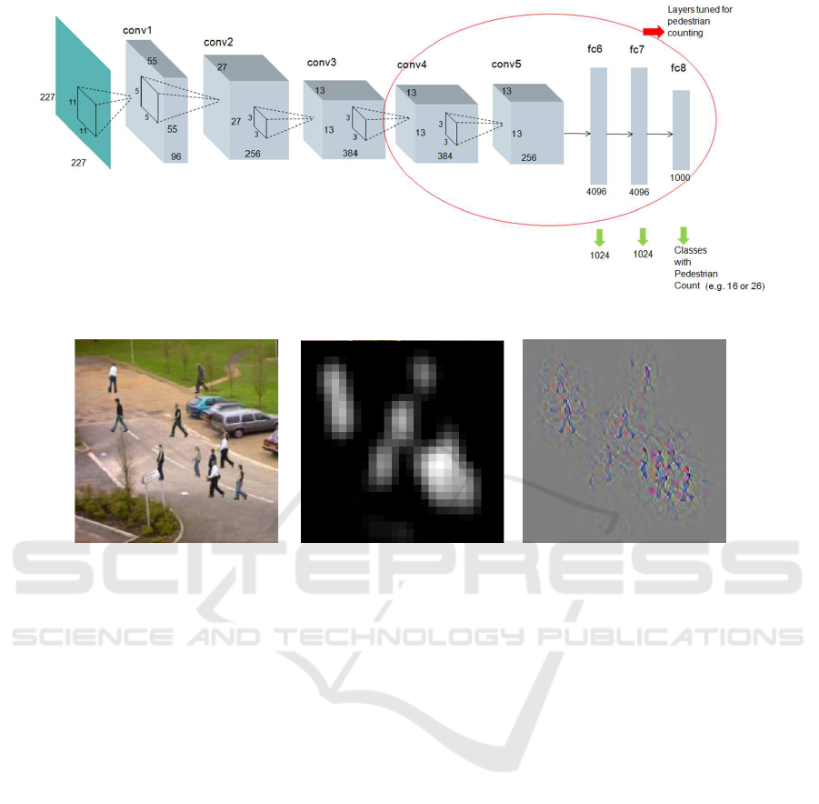
Figure 2: Base network(AlexNet (Krizhevsky et al., 2012)) and its modifications.
(a) Input image. (b) Activation of channel 145
of convolutional layer 5.
(c) Deconvolved output of
channel 145 of convolutional
layer 5.
Figure 3: Visualizing a channel from convolutional layer 5 for a synthetic input image.
Initially, only the classifier, that is, the last fully
connected layer, fc8, was re-trained. The accuracy
improved by fine-tuning the fully connected layers,
fc6 and fc7. It was observed that fine-tuning only fc7
resulted in lesser improvement in performance than
when both fc6 and f7 were fine-tuned. This could
be attributed to the co-adaptation between features
learned in successive layers as described in (Yosinski
et al., 2014). Instead of fine-tuning fc6 and fc7, the
number of nodes were reduced from 4096 to 1024 and
re-trained for a classifier with 16 classes (Count 0 to
15).
By additionally fine-tuning the conv4 and conv5
layers, the accuracy on the validation set increased by
7%. One of the commonly used data augmentation
techniques of taking random crops from the input
image was not used. Since the pedestrians may
be located anywhere in the image, random cropping
from the image might result in the count labels
changing. This would result in an increase in noise of
the target labels. So cropping is avoided. This could
be incorporated provided the count of the pedestrians
in the frame is not affected. Mirroring was used for
augmenting the generated training dataset. The Caffe
(Jia et al., 2014) library was used to train and test the
models for pedestrian counting. Training was carried
out on a Tesla K20 GPU.
3.4 Visualizing Learned Features
In order to understand what the network learns
when trained for pedestrian counting, the learned
filters were visualized using the Deep Visualization
Toolbox (Yosinski et al., 2015). The activations
for the filters in the different layers were observed
along with the features of the input image causing
these activations. The Deep Visualization Toolbox
provides the use of deconvolution as proposed in
(Zeiler and Fergus, 2014) to view the parts of the input
image resulting in activations. Figure 3 shows the
activations of a channel from the fifth convolutional
layer and the corresponding deconvolution results
for a synthetically generated input image from the
validation set. It can be observed that the network
has learned to detect features relevant for counting
pedestrians, like the head, face, the shoulders, torso
VISAPP 2017 - International Conference on Computer Vision Theory and Applications
90

and feet. Additionally, visualizing some of the filters
in the convolutional layers, it is observed that the
network also learns to localize the foreground with
the pedestrians from the background even though this
task was not an explicit goal during the training.
4 EXPERIMENTS
The metric used to measure the performance of the
trained model is mean absolute error (MAE).
MAE =
1
N
N
∑
i=1
|t
i
− y
i
| (5)
where N is the number of test frames, y is the
predicted count of pedestrians and t is the ground
truth or the actual count of pedestrians.
Natural images from the UCSD dataset (Chan
et al., 2008) are used for testing. This dataset has
been completely held out during the training. Square
size crops with varying counts of pedestrians were
taken from the first 2000 frames of the UCSD dataset.
These crops were re-sized to 227x227 before being
used for testing the network. For all subsequent
sections, the MAE values are calculated by taking
the predicted count to be the count corresponding
to the maximum probability. There also exists
the possibility of computing the predicted count as
the average or the weighted average of the top-k
predictions.
4.1 Baseline Model for Pedestrian
Counting
Using the synthetically generated training data, the
network was trained. The weights were initialized
with that from the trained AlexNet model. The
first convolutional layer has a stride of 4 and kernel
size of 11. Due to the stride, blocking artifacts
are present in the learned filters as can be seen
in Figure 4. By reducing the stride in the first
convolutional layer from 4 to 2, the blocking artifacts
are reduced as can be seen in Figure 5. The top-1
validation accuracy increased by 2% by reducing the
stride in the first convolutional layer from 4 to 2.
The above performance was observed by training a
model that did not include any of the background
images (without any pedestrians) of the synthetically
generated images in the training set.
By including the background images in the
training set in the category with zero pedestrians,
the top-1 validation accuracy increased by 4%.
Intuitively, one can think that adding the backgrounds
of the images with pedestrians to the training set
implicitly communicates to the network that it needs
to focus on the pedestrians in its task. A MAE of
1.4 was obtained using test frames from the UCSD
dataset. The test frames were crops fromthe first 2000
frames of the UCSD dataset with limited number
of pedestrians. As can be seen from the Figures 6
and 7 showing the input image on the left and the
probabilities of the classes on the right, it is observed
that the network is able to predict the correct range of
the number of pedestrians, if not the exact pedestrians
even in the complete absence of any training data
from the target set. This shows that the network learns
relevant features for counting pedestrians and is able
to generalize well for a different camera and different
scenes.
In images where the pedestrians have a poor
contrast with the background or when occluded by
other pedestrians, a mis-classification results.
4.2 Direct and Hierarchical Approach
for Enhancing Model Capability
The baseline model was trained to count up to a
maximum of 15 pedestrians in an input frame. To
increase the capability of the model to count up to
a maximum of 25 pedestrians in an input frame,
two different approaches based on transfer learning
were used. In the first case, the direct approach, the
network was initialized with weights from the trained
AlexNet model. In the second case, the hierarchical
approach, the network was initialized with weights
from the baseline pedestrian counting model. In both
cases, the training data set generated synthetically
as described in Section 3.2 was used. The MAE
was found on a test set comprising of frames from
the UCSD dataset. The frames from this test set
are completely held out during the training. As
can be observed from the MAE values in Table 1,
the performance is significantly better in the case
where the network is initialized with weights from the
baseline pedestrian counting model. This is because
AlexNet is trained for categories for the ImageNet
challenge of image classification, which comprise of
very few categories for persons. So the network
when initialized with weights from the AlexNet
model, needs to learn a lot of features relevant for
counting multiple pedestrians. As opposed to this,
the baseline pedestrian counting model has already
learned relevant features for counting pedestrians. To
understandthis phenomenon, all the layers of baseline
model were kept fixed except the last fully connected
layer which was modified to count 25 pedestrians.
Figure 8 shows the visualization of features in the
Pedestrian Counting using Deep Models Trained on Synthetically Generated Images
91

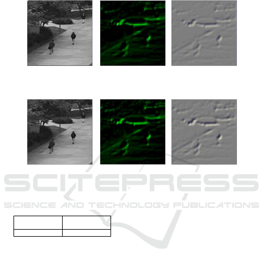
(a) Input image. (b) Activation of a channel of
convolutional layer 1.
(c) Deconvolved output of a
channel of convolutional layer
1.
Figure 4: Blocking artifacts due to stride 4 in convolutional layer 1.
(a) Input image. (b) Activation of a channel of
convolutional layer 1.
(c) Deconvolved output of a
channel of convolutional layer
1.
Figure 5: Blocking artifacts reduction due to stride 2 in convolutional layer 1.
Table 1: Mean absolute error (MAE) for UCSD Dataset
using models with enhanced pedestrian counting capability.
Direct Approach Hierarchical
Approach
3.97 2.86
image causing activations in channel 145 of the conv5
layer of the network using the Deep Visualization
Toolbox. It can be seen that though the count of
pedestrians in the input test image is greater than 15,
the network is still able to find sensible features for
a higher count of pedestrians than it has been trained
for. The hierarchical training method is particularly
suited for pedestrian counting since the categories
of higher counts can be imagined to be supersets
of the lower counts and hence would have some
common features across counts which could be built
on top of what is already learned. The rationale is to
progressively increase the complexity of the training
samples by including more number of pedestrians and
occlusions while building on what the network has
already learned from the simpler training samples.
4.3 Evaluating Cross Entropy and
Squared Error Cost Function
The pedestrian counting model was trained using
two different cost functions, the softmax activation
function with cross entropy (CE) loss along with L
2
regularization and using the linear neuron output with
squared error (SE) loss along with L
2
regularization.
The pairing of the activation function and the cost
function is critical to ensure that rate of convergence
is not affected. (Golik et al., 2013) shows
theoretically and experimentally that the SE loss
function with the softmax activation function has a
lower convergence rate than the CE loss function
with the softmax activation. However, in our case
the SE loss function takes the linear output of the
neuron. Hence, there is no such problem here. Both
softmax with CE and linear neuron output with SE,
havethe cost function gradient with respect to weights
of the final layer that are proportionalto the difference
between the target value and the predicted value as
expressed in equation below.
VISAPP 2017 - International Conference on Computer Vision Theory and Applications
92

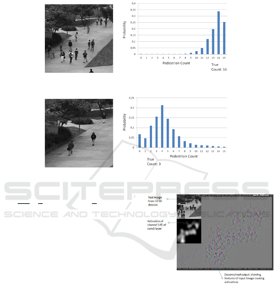
(a) Input image. (b) Classification output.
Figure 6: Classification output for a crop of an image from the UCSD dataset with 16 pedestrians.
(a) Input image. (b) Classification output.
Figure 7: Classification output for a crop of an image from the UCSD dataset with 3 pedestrians.
∂L
∂w
L
jk
=
1
N
N
∑
i=1
(y
L
ij
− t
ij
)y
L−1
ik
+
λ
N
kw
L
jk
k
2
(6)
where, L denotes the output layer, w
L
jk
denotes the
weight between node j of layer L and node k of layer
L − 1, y
L
ij
denotes the predicted output for training
example i at node j of the output layer, t
ij
denotes
the target output for training example i at node j of
the output layer and y
L−1
ik
denotes the output of node
k of layer L − 1 for training example i. As can be
observed, there are no higher order terms that may
result in smaller values of the gradient even when
the output is of a value with the opposite sign (Golik
et al., 2013).
It was observed that the network trained using
synthetically generated images and CE loss performs
significantly better than the one trained using SE loss
when tested on natural images not experienced by the
model during training. The model trained using the
SE loss function resulted in a MAE of 5.05 while
the model trained using CE loss resulted in a MAE
of 2.86 on the UCSD dataset. A reason for the SE
cost function resulting in poorer performance than
the CE cost function is the sensitivity of the SE
cost function to noise in training data and outliers.
The training data has noisy labels in cases where the
frames of the sequence have some of the pedestrians
Figure 8: Deconvolved result of a frame from the UCSD
Dataset with around 25 pedestrians using the feature
extractor of the baseline model (generated using Deep
Visualization Toolbox).
moving out of the scene or if some of the pedestrians
are completely occluded and the count does not get
updated. Other sources of noise are from the merging
of the foreground with the background and noise
present in the elements of the natural images used
to compose the synthetic images. The implication is
that the trained model generalizes poorly in the case
of SE cost function since it is not robust to noise.
Kline et al. (Kline and Berardi, 2005) highlight the
sensitivity of the SE cost function to noise as one of
Pedestrian Counting using Deep Models Trained on Synthetically Generated Images
93

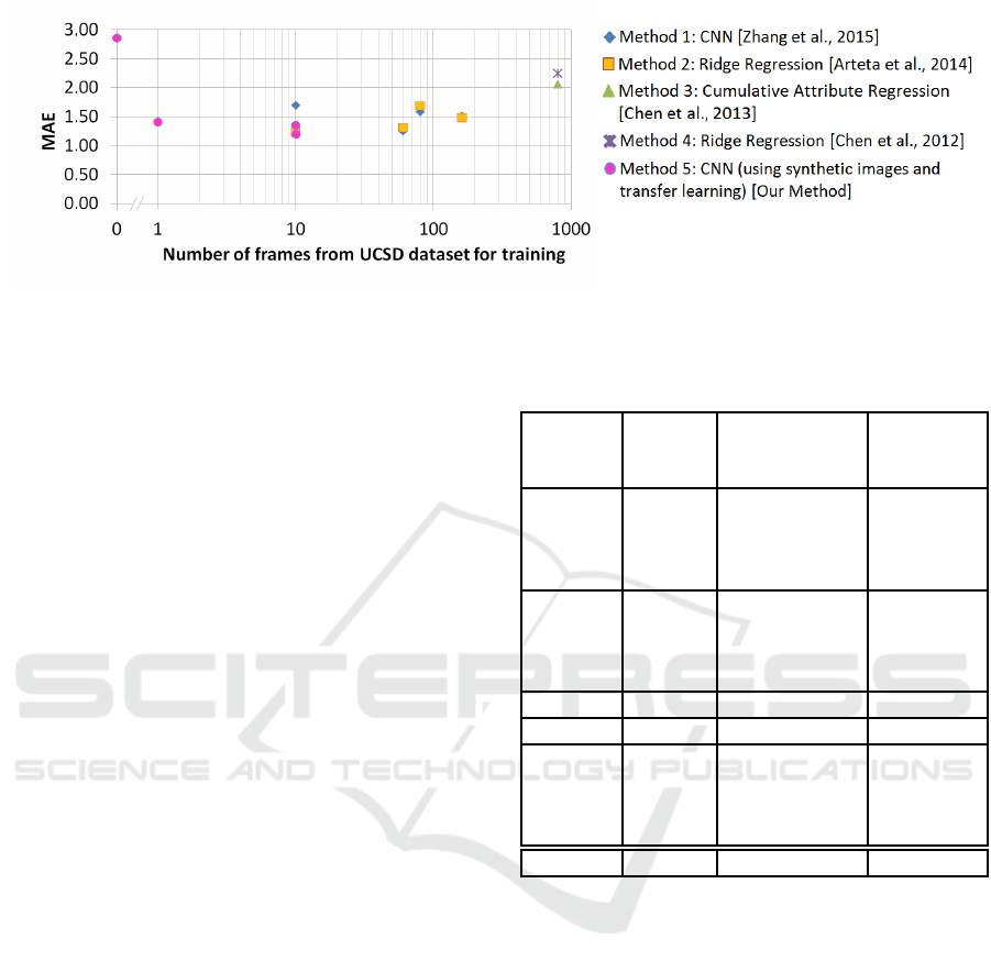
Figure 9: Comparing MAE values with respect to the number of frames used from the target dataset (UCSD) for training.
the factors in the analysis of the benefits of the CE
cost function over the squared error cost function.
(Moody, 1991) indicates that there is an increased
generalization error with increased noise. Using CE
as the loss function gives a better performance than
the squared error loss function for a model trained
entirely on synthetically generated training data and
being tested on natural images not seen be the model
during training. In this scenario, generalization plays
a critical role while the presence of noise in the
training data and the sensitivity of the cost function
to noise can adversely affect the performance of the
model.
Moreover, the advantage of using the CE loss
(classification) is that we get an indication of the
range of possible values along with the probability.
A unimodal histogram is an indication of a good
estimate while a multimodal estimate should be less
trusted. Moreover when using SE loss (regression), it
is possible that the predicted value is not within the
valid range of values.
4.4 Comparison with Other Pedestrian
Counting Approaches
Table 2 shows the MAE values on the UCSD dataset
using different pedestrian counting methods reported
in literature (Methods 1 - 4 and 6) and our method
(Method 5). All of the methods reported in literature
use frames from the UCSD dataset for training.
Table 2 indicates the number of frames from the
UCSD dataset being used along with the duration
and interval of frames from the sequence for training.
Figure 9 is a scatter plot useful for comparing the
MAE values of Table 2 with respect to the number
of frames used from the UCSD dataset for training
for Methods 1 to 5. The specifics of Method 1-5
of Table 2 are mentioned in the legend of Figure 9
and should be viewed in conjunction. (Zhang et al.,
2015) trains a crowd counting model and achieves
Table 2: Comparison with other pedestrian counting
approaches for the UCSD dataset.
Method
†
Count
(of
frames)
Start:Step:Stop
(frame
number)
MAE
1 160 600:5:1400 1.7
80 1205:5:1600 1.26
60 805:5:1100 1.59
10 640:80:1360 1.52
2 160 600:5:1400 1.24
80 1205:5:1600 1.31
60 805:5:1100 1.69
10 640:80:1360 1.49
3 800 600:1400 2.07
4 800 600:1400 2.25
5 0 2.86
1 1.41
10 20:20:200 1.36
10 620:20:800 1.20
6 * * 0.74
* (Segui et al., 2015) Synthetic images generated by
extracting pedestrians from UCSD dataset and placing
them against the background of UCSD dataset for training.
MAE value on test set from UCSD dataset.
† The specifics of Method 1-5 are in the legend of Figure 9
and should be viewed in conjunction.
the best MAE of 1.26 on the UCSD dataset for the
’downscale’ mode which comprises of training on
frames 1205:5:1600. This duration of the sequence
comprises of the highest density and number of
pedestrians in the sequence. The test frames for
the rest of the sequence comprise lesser number of
pedestrians.
For our case, the model does not experience any
natural images from the target dataset or otherwise.
In fact the model does not experience the images from
the same camera or scene as that of the target dataset
during training. The MAE for a maximum of 25
pedestrians per crop of a frame for the UCSD dataset
VISAPP 2017 - International Conference on Computer Vision Theory and Applications
94

Figure 10: Predictions on crops of vidf1 33 01 of UCSD dataset.
is 2.86. If our pedestrian counting model is fine-tuned
using only the background of the target dataset, there
is a significant improvement in the performance. The
model was fine-tuned by introducing the background
of the UCSD dataset in class 0 of the training data
and letting the other classes use synthetic data to
have class balancing. The result is an improved
MAE of 1.41 in place of 2.86 and is comparable
with the results obtained by other state-of-the-art
approaches. By additionally using 10 frames with
pedestrians from the UCSD dataset (from the frame
interval 20 to 200), the MAE for our method improves
further to 1.36. Instead of frame interval 20 to
200, if frame interval 620 to 800 is used which has
more dense groups of pedestrians, the MAE for our
method further improves to 1.20. The graph in Figure
10 shows for crops of the sequence ’vidf1
33 001’
(from the UCSD data set) with 200 frames, the
actual and estimated pedestrian count using a model
trained completely on synthetically generated images
and the improvement in the estimate obtained by
finetuning using the background of the dataset. (Segui
et al., 2015) trains a CNN using images generated
by extracting pedestrians from the UCSD dataset
and merging them with the background of the
UCSD dataset. Each frame has a maximum of 25
pedestrians. The MAE obtained for such a setup for
the UCSD dataset was 0.74. Since the background
and foregrounds used to generate the training images
are both obtained from the UCSD dataset and the test
images are also from the same dataset, the MAE is a
very low value. Hence this method listed as Method
6 in Table 2 is not plotted in Figure 9.
5 CONCLUSION
We present a novel approach for pedestrian counting
based on training deep models using synthetically
generated images and transfer learning. When there
is a lack of sufficient annotated training data or
perhaps none, for example, in the scenario where
the camera is under development or the target site
is inaccessible, it is a practical solution to deploy
the model and still obtain meaningful results. After
setting up the system, it is feasible to capture a
few images of the background for fine-tuning. The
suitability of the cross entropy cost function was
established for this scenario. This approach is able to
achieve a generalization across multiple dimensions:
acquisition devices for the same imaging modality,
scenes and from synthetic to natural images. Transfer
learning is systematically used at three steps: to
create the baseline model using only synthetic data,
the enhanced model from the baseline model using
only synthetic data and finally the improved model
using additionally the background or few images
from the target site. Annotation efforts are not
required if the training data is generated synthetically.
Since no explicit detection of pedestrians is done,
the training annotations are simple, requiring only a
single number. With transfer learning, the models
can be generated quickly thus avoiding a full-fledged
lengthy training with a large amount of training data.
Some of the next steps include using better
synthetic data generation models considering aspects
like illumination and using sequences of image
frames to improve the performance of the existing
models for the target dataset.
Pedestrian Counting using Deep Models Trained on Synthetically Generated Images
95

ACKNOWLEDGEMENTS
The research leading to these results has received
funding from the German Federal Ministry
for Economic Affairs and Energy under the
VIRTUOSE-DE project.
REFERENCES
Andriluka, M., Roth, S., and Schiele, B.
(2008). People-tracking-by-detection and
people-detection-by-tracking. In IEEE Conference
on Computer Vision and Pattern Recognition, 2008.
CVPR 2008., pages 1–8.
Angelova, A., Krizhevsky, A., and Vanhoucke, V. (2015a).
Pedestrian detection with a large-field-of-view deep
network. In Proceedings of ICRA 2015.
Angelova, A., Krizhevsky, A., Vanhoucke, V., Ogale, A.,
and Ferguson, D. (2015b). Real-time pedestrian
detection with deep network cascades. In Proceedings
of BMVC 2015.
Arteta, C., Lempitsky, V., Noble, J. A., and Zisserman, A.
(2014). Interactive Object Counting, pages 504–518.
Springer International Publishing, Cham.
Baltieri, D., Vezzani, R., and Cucchiara, R. (2011). 3dpes:
3d people dataset for surveillance and forensics. In
Proceedings of the 1st International ACM Workshop
on Multimedia access to 3D Human Objects, pages
59–64, Scottsdale, Arizona, USA.
Bengio, I. G. Y. and Courville, A. (2016). Deep learning.
Book in preparation for MIT Press.
Chan, A. B., Liang, Z.-S. J., and Vasconcelos, N. (2008).
Privacy preserving crowd monitoring: Counting
people without people models or tracking. In
Computer Vision and Pattern Recognition, 2008.
CVPR 2008. IEEE Conference on, pages 1–7.
Chan, A. B., Morrow, M., and Vasconcelos, N.
(2009). Analysis of crowded scenes using holistic
properties. In Performance Evaluation of Tracking
and Surveillance workshop at CVPR 2009, pages
101–108, Miami, Florida.
Chen, K., Gong, S., Xiang, T., and Loy, C. C. (2013).
Cumulative attribute space for age and crowd density
estimation. In 2013 IEEE Conference on Computer
Vision and Pattern Recognition, Portland, OR, USA,
June 23-28, 2013, pages 2467–2474.
Chen, K., Loy, C. C., Gong, S., and Xiang, T. (2012).
Feature mining for localised crowd counting. In
British Machine Vision Conference, BMVC 2012,
Surrey, UK, September 3-7, 2012, pages 1–11.
Enzweiler, M. and Gavrila, D. M. (2009). Monocular
pedestrian detection: Survey and experiments. IEEE
Transactions on Pattern Analysis and Machine
Intelligence, 31(12):2179–2195.
Fiaschi, L., Koethe, U., Nair, R., and Hamprecht, F. A.
(2012). Learning to count with regression forest and
structured labels. In 21st International Conference on
Pattern Recognition (ICPR), 2012, pages 2685–2688.
Fujii, Y., Yoshinaga, S., Shimada, A., and ichiro Taniguchi,
R. (2010). The 1st international conference on
security camera network, privacy protection and
community safety 2009 real-time people counting
using blob descriptor. Procedia - Social and
Behavioral Sciences, 2(1):143 – 152.
Girshick, R. B., Donahue, J., Darrell, T., and Malik,
J. (2013). Rich feature hierarchies for accurate
object detection and semantic segmentation. CoRR,
abs/1311.2524.
Golik, P., Doetsch, P., and Ney, H. (2013). Cross-entropy
vs. squared error training: a theoretical and
experimental comparison. In Interspeech, pages
1756–1760, Lyon, France.
Hattori, H., Naresh Boddeti, V., Kitani, K. M., and
Kanade, T. (2015). Learning scene-specific pedestrian
detectors without real data. In The IEEE Conference
on Computer Vision and Pattern Recognition (CVPR).
Hinton, G. E., Srivastava, N., Krizhevsky, A., Sutskever,
I., and Salakhutdinov, R. (2012). Improving neural
networks by preventing co-adaptation of feature
detectors. CoRR, abs/1207.0580.
Jia, Y., Shelhamer, E., Donahue, J., Karayev, S., Long,
J., Girshick, R., Guadarrama, S., and Darrell, T.
(2014). Caffe: Convolutional architecture for fast
feature embedding. arXiv preprint arXiv:1408.5093.
Kline, M. and Berardi, L. (2005). Revisiting squared-error
and cross-entropy functions for training neural
network classifiers. Neural Comput. Appl.,
14(4):310–318.
Krizhevsky, A., Sutskever, I., and Hinton, G. E. (2012).
Imagenet classification with deep convolutional
neural networks. In Advances in Neural Information
Processing Systems 25: 26th Annual Conference
on Neural Information Processing Systems 2012.
Proceedings of a meeting held December 3-6,
2012, Lake Tahoe, Nevada, United States., pages
1106–1114.
LeCun, Y., Bengio, Y., and Hinton, G. (2015). Deep
learning. Nature, 521(7553):436–444.
Lempitsky, V. and Zisserman, A. (2010). Learning to count
objects in images. In Lafferty, J. D., Williams, C.
K. I., Shawe-Taylor, J., Zemel, R. S., and Culotta, A.,
editors, Advances in Neural Information Processing
Systems 23, pages 1324–1332. Curran Associates, Inc.
Liu, W., Wen, Y., Yu, Z., and Yang, M. (2016).
Large-margin softmax loss for convolutional neural
networks. In ICML.
Luo, P., Wang, X., and Tang, X. (2013). Pedestrian
parsing via deep decompositional network. In IEEE
International Conference on Computer Vision, ICCV
2013, Sydney, Australia, December 1-8, 2013, pages
2648–2655.
Merad, D., Aziz, K. E., and Thome, N. (2010). Fast people
counting using head detection from skeleton graph. In
Seventh IEEE International Conference on Advanced
Video and Signal Based Surveillance (AVSS), 2010,
pages 151–156.
Moody, J. E. (1991). The effective number of parameters:
An analysis of generalization and regularization in
VISAPP 2017 - International Conference on Computer Vision Theory and Applications
96

nonlinear learning systems. In Advances in Neural
Information Processing Systems 4, [NIPS Conference,
Denver, Colorado, USA, December 2-5, 1991], pages
847–854.
Overett, G., Petersson, L., Brewer, N., Andersson, L.,
and Pettersson, N. (2008). A new pedestrian dataset
for supervised learning. In Intelligent Vehicles
Symposium, 2008 IEEE, pages 373–378.
Richter, S. R., Vineet, V., Roth, S., and Koltun, V. (2016).
Playing for data: Ground truth from computer games.
In Leibe, B., Matas, J., Sebe, N., and Welling, M.,
editors, European Conference on Computer Vision
(ECCV), volume 9906 of LNCS, pages 102–118.
Springer International Publishing.
Ros, G., Sellart, L., Materzynska, J., Vazquez, D., and
Lopez, A. M. (2016). The synthia dataset: A
large collection of synthetic images for semantic
segmentation of urban scenes. In The IEEE
Conference on Computer Vision and Pattern
Recognition (CVPR).
Segui, S., Pujol, O., and Vitria, J. (2015). Learning to count
with deep object features. In The IEEE Conference
on Computer Vision and Pattern Recognition (CVPR)
Workshops.
Vezzani, R. and Cucchiara, R. (2010). Video surveillance
online repository (visor): an integrated framework.
Multimedia Tools and Applications, 50(2):359–380.
Yosinski, J., Clune, J., Bengio, Y., and Lipson, H.
(2014). How transferable are features in deep neural
networks? In Advances in Neural Information
Processing Systems 27, pages 3320–3328. Curran
Associates, Inc.
Yosinski, J., Clune, J., Nguyen, A., Fuchs, T., and
Lipson, H. (2015). Understanding neural networks
through deep visualization. In Deep Learning
Workshop, International Conference on Machine
Learning (ICML).
Yu, Z., Gong, C., Yang, J., and Bai, L. (2014). Pedestrian
counting based on spatial and temporal analysis.
In 2014 IEEE International Conference on Image
Processing (ICIP), pages 2432–2436.
Zeiler, M. D. and Fergus, R. (2014). Visualizing
and understanding convolutional networks. In
Computer Vision - ECCV 2014 - 13th European
Conference, Zurich, Switzerland, September 6-12,
2014, Proceedings, Part I, pages 818–833.
Zhang, C., Li, H., Wang, X., and Yang, X. (2015).
Cross-scene crowd counting via deep convolutional
neural networks. In 2015 IEEE Conference on
Computer Vision and Pattern Recognition (CVPR),
pages 833–841.
Zhao, H., Gallo, O., Frosio, I., and Kautz, J. (2015). Loss
Functions for Neural Networks for Image Processing.
ArXiv e-prints 1511.08861.
Pedestrian Counting using Deep Models Trained on Synthetically Generated Images
97