Coupled 2D and 3D Analysis for Moving Objects Detection with a
Moving Camera
Marie-Neige Chapel, Erwan Guillou and Saida Bouakaz
Universit
´
e de Lyon, CNRS, Universit
´
e Lyon 1, LIRIS, UMR5205, F-69622, Lyon, France
Keywords:
Object Detection, Moving Camera, 3D Geometric Constraint, Statistical Analysis.
Abstract:
The detection of moving objects in the video stream of a moving camera is a complex task. Static objects
appear moving in the video stream as moving objects. Thus, it is difficult to identify motions that belong to
moving objects because they are hidden by those of static objects. To detect moving objects we propose a
novel geometric constraint based on 2D and 3D information. A sparse reconstruction of the visible part of the
scene is performed in order to detect motions in the 3D space where the scene perception is not deformed by
the camera motion. A first labeling estimation is performed in the 3D space and then apparent motions in the
video stream of the moving camera are used to validate the estimation. Labels are computed from confidence
values which are updated at each frame according to the geometric constraint. Our method can detect several
moving objects in complex scenes with high parallax.
1 INTRODUCTION
Nowadays, using visual effects is common in movies.
These are integrated during the post-production stage
and the director can only guess the final result during
shooting. In order to help the director in his task, a
preview of the final result render could be provided
onset. It requires to combine virtual elements (visual
effects) and real ones, with spatial and temporal co-
herence. Since we cannot add markers to moving ob-
jects, it is necessary to detect them in the video stream
of the camera.
In this paper we propose a method to detect mov-
ing objects without any marker in the stream of a free
moving camera. The scene contains a static part and
a moving part where we distinguish two types of mo-
tions: the apparent motion: objects are static, but
appear to be moving because of the camera motion;
the real motion: objects are moving in the scene and
this motion is captured by the camera. The apparent
motions of the scene can be uniform or non-uniform
according to the scene setup and the camera motion.
The apparent motion of an object in the scene depends
on its distance to the camera and the camera motion.
It is difficult to identify apparent motions generated
by static objects and those that come from to mov-
ing objects when the camera film moving objects in
a static scene. Moreover, as the camera moves, some
parts of the scene become visible while some other
are occluded. Thus, it is necessary to compute and
include new information in the process of moving ob-
ject detection throughout the video sequence.
The contribution of this paper is a novel geomet-
ric constraint based on feature points extracted from
video frames. The geometric constraint relies on 2D
and 3D information to perform a robust moving ob-
ject detection in the video stream of a moving cam-
era. This geometric constraint is based on a set of
static points used as a geometric reference to update
all feature point labels. When the camera moves, the
reference set has to be updated during the sequence
by adding and removing feature points.
The remainder of this paper is organized as fol-
lows: Section 2 reviews previous work related to
moving object detection; details of the proposed
method are sketched in Section 3; experimental re-
sults are described in Section 4; finally we conclude
the paper and provide future directions in Section 5.
2 STATE OF THE ART
Detecting and tracking moving objects in video has
been widely studied over the last decades. Various
object detection approaches are reported in the litera-
ture. Moving object detection with a stationary cam-
era usually relies on background subtraction, (Sobral
and Vacavant, 2014). A background model is de-
236
Chapel M., Guillou E. and Bouakaz S.
Coupled 2D and 3D Analysis for Moving Objects Detection with a Moving Camera.
DOI: 10.5220/0006132002360245
In Proceedings of the 12th International Joint Conference on Computer Vision, Imaging and Computer Graphics Theory and Applications (VISIGRAPP 2017), pages 236-245
ISBN: 978-989-758-227-1
Copyright
c
 2017 by SCITEPRESS – Science and Technology Publications, Lda. All rights reserved

scribed by a statistical model based on pixel charac-
teristics. The current image is then compared to the
background model to detect moving objects and the
background model is updated. Proposed approaches
differ by elimination of noise due to shadows or illu-
mination changes for example.
The context of the movie industry requires using
moving cameras. Approaches that dealt with moving
object detection in the stream of a moving camera can
be divided into three categories.
The first category of method uses motions to de-
tect moving objects. In the video stream of a freely
moving camera, the static background appears mov-
ing. Trajectory segmentation methods try to segment
trajectories that belong to the static scene and those
that belong to moving objects. Methods proposed
by Elqursh et al. (Elqursh and Elgammal, 2012) and
Ochs et al. (Ochs et al., 2014) cluster trajectories us-
ing their location, magnitude and direction. Elqursh
et al. (Elqursh and Elgammal, 2012) label clusters as
static or moving according to criteria such as com-
pactness or spatial closeness, and propagate label in-
formation to all pixels with a graph-cut on an MRF.
Ochs et al. (Ochs et al., 2014) merge clusters ac-
cording to the mutual fit of their affine motion models
and label information are propagated with a hierar-
chical variational approach based on color and edge
information. Sheikh et al. (Sheikh et al., 2009) rep-
resent the background motion by a subspace based
on three trajectories selectionned in the optical flow.
Each trajectory is assigned to the background or the
foreground depending on the trajectory fits to the
subspace or not. Narayana et al. (Narayana et al.,
2013) use a translational camera and exploit only
optical flow orientations which are independent of
depth. Based on a set of pre-computed orientation
fields for different motion parameters of the camera,
the method automatically detects the number of fore-
ground motions. Methods based on trajectory seg-
mentation generally assume that the apparent motion
of the scene is predominant and uniform but this is not
always true.
Another category of approach uses the back-
ground subtraction techniques with a moving camera.
Using a moving camera with constrained motions al-
lowed to construct a background model of the scene.
Each frame is then registered with the background
model to perform the background subtraction. The
Pan Tilt Zoom (PTZ) camera is a constrained mov-
ing camera with a fixed optical center. The key prob-
lem to perform background subtraction is to regis-
ter the camera image with the panoramic background
model at different scale. Xue et al. (Xue et al., 2013)
proposed a method that relies on a panoramic back-
ground model and a hierarchy of images of the scene
at different scales. A match is found between the
current image and images in the hierarchy, then the
match is propagated to upper level until registration
with the panoramic background. Cui et al. (Cui et al.,
2014) use a static camera to capture large-view im-
ages at low resolution to detect motions in order to
define a rough region with the moving object. The
high resolution image of the PTZ camera is registered
with the background model with feature point match-
ing and refines with an affine transformation model.
Background subtraction techniques can also be used
with a freely moving camera. In general, the cam-
era motion is compensated with a homography, but
when the camera undergoes a translational motion
some misalignments created by parallax can be de-
tected as moving object. Romanoni et al. (Romanoni
et al., 2014) and Kim et al. (Kim et al., 2013) used
a spatio-temporal model to classify misaligned pixels
relying on neighborhood analysis. Instead of regis-
tering the whole image, the method proposed by Yi
et al. (Yi et al., 2013) divided the image into grids,
each grid being described by a single gaussian model.
To keep the background model up-to-date, each block
at previous time is mixed with blocks in the current
image after registration. Two background models are
maintained to prevent foreground contamination. All
these approaches handled scenes with uniform appar-
ent motion of background but failed when the camera
films a complex scene closely.
The last category of methods approximating the
scene by one or several planes are Plane+Parallax
and multi-plane approaches. According to the mo-
tion of a freely moving camera, motions of two static
objects observed in the video stream can have differ-
ent magnitudes and orientations. The Plane+Parallax
methods extend the plane approximation by taking
into account the parallax. Some work have first ap-
proximated the scene by a plane (Irani and Anan-
dan, 1998; Sawhney et al., 2000; Yuan et al., 2007).
This plane is the physical dominant plane in the im-
ages and called the reference plane. After register-
ing consecutive images according to the reference
plane, the misaligned points are due to parallax. In
order to label these points as moving or static, the
authors propose geometric constraints based on the
reference plane. The Plane+Parallax methods only
handle scenes that can be approximated by one dom-
inant plane as aerial images. To be more general, the
multi-layer approaches approximate the scene by sev-
eral virtual or physical planes. Wang et al. (Wang and
Adelson, 1994) propose that each layer contains an
intensity map, an alpha map and a velocity map. The
optical flow is segmented with k-means clustering.
Coupled 2D and 3D Analysis for Moving Objects Detection with a Moving Camera
237

Thus, each layer contains a smooth motion field and
accumulates information corresponding to its motion
field over time. Jin et al. (Jin et al., 2008) generate
a layer for each physical plane. The Random Sam-
ple Consensus (RANSAC) is performed iteratively
on the set of feature points, previously matched be-
tween two frames. The current frame is then recti-
fied with homographies found by RANSAC for each
physical plane for background modeling. Zamalieva
et al. (Zamalieva and Yilmaz, 2014) discretize the
scene with a set of hypothetical planes. A physi-
cal plane is selected arbitrarily as a reference plane
and parallel and equidistant hypothetical planes are
generated from the reference plane. A background
model is maintained for each hypothetical plane and
pixels are labeled as background by maximizing the
a posteriori probability. Zamalieva et al. proposed
another method (Zamalieva et al., 2014) that selects
the transformation that best describes the geometry
of the scene. A modified Geometrical Robust Infor-
mation Criterion (GRIC) score is computed to choose
between the homography when the scene can be ap-
proximated by one plane or the fundamental matrix
for several planes. The image is segmented into fore-
ground/background with motion, appearance, spatial
and temporal cues. Plane+Parallax methods assume
there is a dominant plane in the scene like aerial im-
agery. Using a dominant plane in Plane+Parallax or
in multi-planes methods, generally supposes that the
plane has to be in the field of view of the camera
over the whole sequence. Multi-planes methods ap-
proximating the scene by several planes suffer from
low performance when there is significant parallax
because of the granularity of the scene representation.
To the best of our knowledge, proposed ap-
proaches to detect moving objects in the video stream
of a moving camera cannot handle complex scenes
when the camera is close to the scene. In this case,
and without prior knowledge, it is difficult to deal
with complex apparent motions or the granularity of
the scene representation. In this paper, we present
a method which goes further than multi-layer ap-
proaches by computing a sparse scene reconstruction.
As the Plane+Parallax method, we propose to use
a geometric constraint, but unlike this approach the
constraint does not rely on a plane but on several 3D
points belonging to the static part of the scene. We
also use apparent motions as a validation step of the
labeling.
3 PROPOSED METHOD
Our goal is to detect moving objects in the video
stream of a freely moving camera. The intrinsic pa-
rameters of the moving camera are assumed to be
known. Our method works on feature points ex-
tracted and tracked with the Large Displacement Op-
tical Flow (LDOF) algorithm (Brox and Malik, 2011).
Each feature point is described by a 2D image posi-
tion p, an optical flow vector f over ∆t frames, a 3D
position P and a confidence value Con f . The confi-
dence value is a real value between −1 and 1. Each
feature point is labeled as moving or static depending
if its confidence value is close to −1 or 1 respectively.
l
i
=



moving if Con f
i
< ε
moving
static if Con f
i
> ε
static
unknown otherwise
(1)
with ε
moving
∈ [−1, 0] and ε
static
∈ [0, 1]. These val-
ues are choosen from experiments for each sequence.
Confidence values close to zero are not considered
distinctive enough to decide between static and mov-
ing label and we thus introduced a third label: un-
known.
The update of the confidence value is based on a
3D geometric constraint over time. Let P
t
be the set
of all feature points at time t. Static points of the scene
can be assimilated to a rigid body noted N
t
⊂ P
t
. In
a rigid body, distances between any two points must
remain constant over time. Hence, a new feature point
that appears in the video stream of the camera at time
t − ∆t is part of N
t
if its distance to any point of N
t
remains constant over ∆t frame. This defines our ge-
ometric constraint that is used to update confidence
values over time. All feature points labeled as static
at time t define a rigid body N
t
used as reference to
update confidence values for the next frame.
Since the geometric constraint is defined in 3D
space, it is necessary to estimate the 3D position of
feature points. Thanks to point matching provided
by the LDOF algorithm and the known intrinsic ma-
trix, it is possible to reconstruct 3D positions of fea-
ture points from 2D information by approximating the
camera motion. The essential matrix is computed us-
ing the method proposed by Nist
´
er (Nist
´
er, 2004) on
the rigid body N
t
. Then, the confidence value of a
feature point increases or decreases according to the
geometric constraint.
Before detecting moving objects, an initialisation
step is performed to estimate the first set of static
points. To test the 3D geometric constraint, 3D po-
sitions of feature points are computed by estimating
the essential matrix on feature points belonging to
N
t−∆t
∩ N
t
for two consecutive frames. Then, confi-
dence values are updated to obtain a new labelisation.
Finally, a label validation is performed using 2D in-
formation.
VISAPP 2017 - International Conference on Computer Vision Theory and Applications
238

3.1 Reconstruction Scaling
Our 3D geometric constraint expresses the character-
istic of a rigid body by comparing distances between
points from two reconstructions of two consecutives
frames. However, the essential matrix used for the
reconstruction of the scene is estimated up to a scale
factor depending on the camera motion. Hence the
scale of the reconstruction differs over time. Let R
be the exact reconstruction, which is not known. Let
R
t
be the reconstruction obtained using the method of
Nist
´
er (Nist
´
er, 2004) at time t with R
t
' s
t
R . Since
we need to compare 3D distances over time to com-
pute our geometric constraint, we need two similar
reconstructions with the same scale factor. To make
a reconstruction R
t
comparable with a previous one
R
t−∆t
, we have to estimate s and apply it to R
t
. First,
we estimate the ratio s
i, j
of distances between two
points i and j as:
s
i, j
=
dist(P
i
− P
j
)
t−∆t
dist(P
i
− P
j
)
t
, P
i
, P
j
∈ N
t−∆t
∩ N
t
(2)
Since the feature point extraction is in general
noisy, it would be unreliable to estimate the scale fac-
tor from only two points. To suppress peak noise and
choose the best scale factor, we compute the median
scale factor for each feature point as:
s
i
= median(s
i, j
) (3)
The scale factor s applied to R
t
is then defined as
the median of all scale factors of feature points:
s = median(s
i
) (4)
The reconstruction at frame t is scaled with pre-
vious ones using s. Thus, the reconstruction sR
t
at
time t can be compared with a previous one in order
to update the confidence value.
3.2 Labeling Update
At each frame, the geometric constraint is tested for
each feature point in order to update its confidence
value. The geometric constraint states that 3D dis-
tances between a point P
i
and all points in N remains
constant between two reconstructions at t and t − ∆t.
∆t is chosen big enough to let moving objects to move
during ∆t time and small enough to track a lot of fea-
ture points. N is divided into two subsets V and I
for each feature point P
i
as follows:
V
t
= {P
t
j
|P
t
j
∈ N
t
, Err(P
i
, P
j
)
t
< ε
err3D
}
I
t
= N
t
\V
t
(5)
where ε
err3D
is defined from experiments and Err
defines the distance error between two frames as:
Err(P
i
, P
j
)
t
= |dist(P
i
, P
j
)
t
− dist(P
i
, P
j
)
t−∆t
| (6)
and ε
err3D
is the threshold on distance errors to
differentiate a static point from a moving one. V
t
refers to the subset of N
t
for which the geometric
constraint, defined by Equation (6), is verified and I
t
its complement.
These two subsets are used to update the confi-
dence value of P
i
as follows:
Con f
t
i
= Con f
t−1
i
+U
t
i
(7)
where Con f
t
i
∈ [−1, 1] and U
t
is an update value
that is different according to the estimate state of the
feature point as explained below.
Static Point Update. A feature point P
t
i
is esti-
mated static over [t, t − ∆t] if |V
t
i
| > α|N
t
| where
α ∈ [0, 1] defines the proportion of N for which P
t
i
verifies the geometric constraint. The level of cer-
tainty for which P
t
i
is estimated static is defined by
the mean error Err
t
i
of distance errors on V
Err
t
i
=
1
|V
t
i
|
∑
P
j
∈V
t
i
Err(P
i
, P
j
)
t
(8)
From V defines in (5), Err
t
i
∈ [0, ε
err3D
|. A mean
error close to 0 implied a high level of certainty on
the rigid body conservation. In this case, the point has
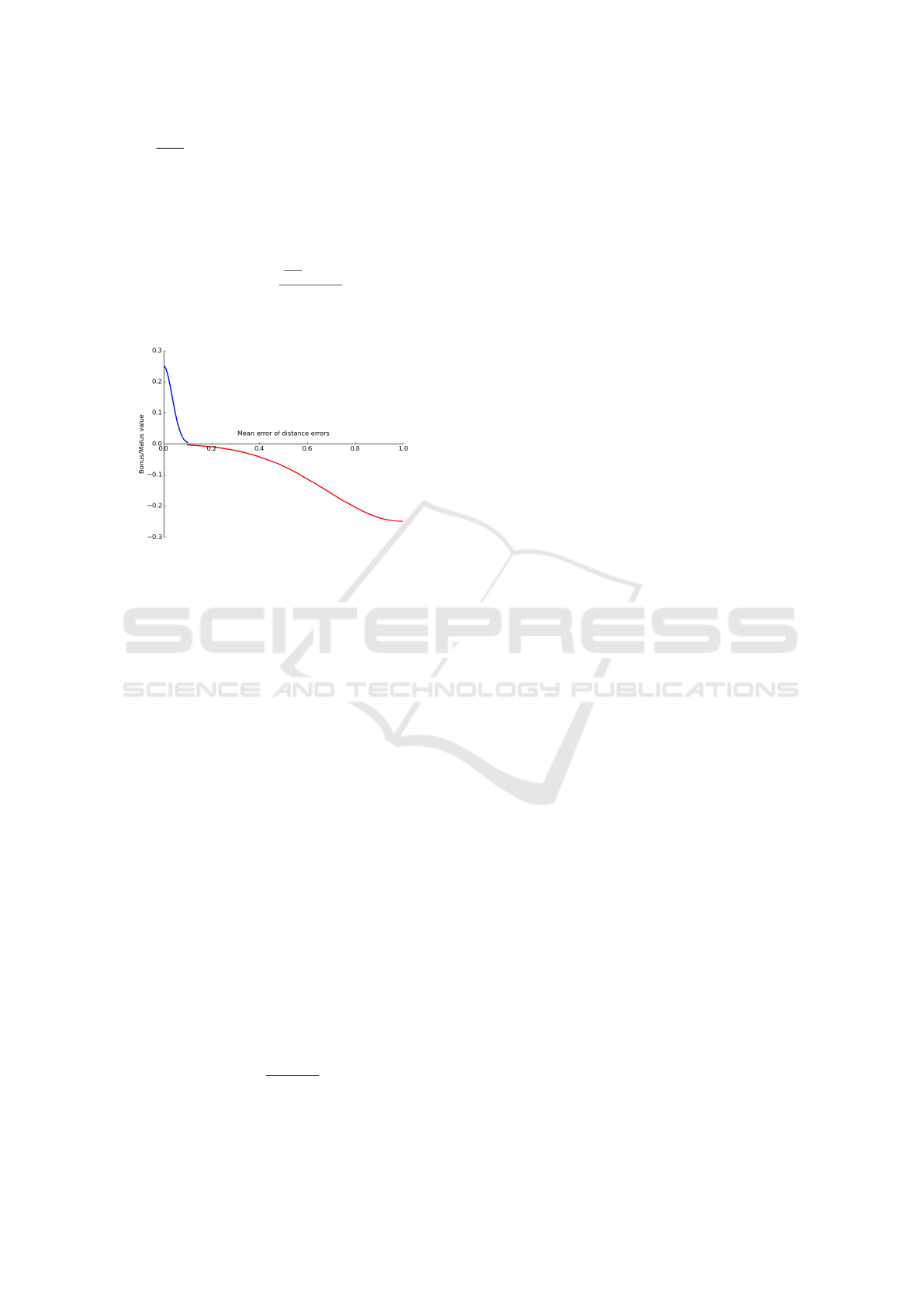
to be immediately updated tostatic. On the contrary,
for a mean error closed to ε
err3D
the level of certainty
is low and the update value has a low impact on the
confidence value. This behavior is depicted in figure
1 and defined as follows:
U
t
i
= re
−
Err
t
i
ε
err3D
!
2
(9)
where r ∈ [0, 1] is a coefficient that defines the
minimum number of frames necessary to label the
feature point as static. The update value is defined
over [t, t − ∆t] and modifies the confidence value
which progresses over the whole sequence to a static
labeling.
Moving Point Update. Conversely to the previous
case, a feature point P
t
i
is estimated as moving over
[t,t −∆t] if |V
t
i
| < α|N
t
|. The level of certainty is the
mean error of distance errors on I
Err
t
i
=
1
|I
t
i
|
∑
P
j
∈I
t
i
Err(P
i
, P
j
)
t
(10)
Coupled 2D and 3D Analysis for Moving Objects Detection with a Moving Camera
239

where Err
t
i
∈ [ε
err3D
, max
err
] and max
err
is a parame-
ter to discard large distance errors. If Err(P
i
, P
j
)
t
>
max
err
then we considered that Err(P
i
, P
j
)
t
= max
err
.
Since the feature point is estimated as moving, the up-
date value U
t
i
has to be negative and adjusted accord-
ing to the level of certainty as follows:
U
t
i
= −re
−
Err
t
i
−max
err
max
err
−ε
err3D
!
2
(11)
where r is defined as in the static case.
Figure 1: Curves of update values for a static point (blue)
and a moving point (red). Here r = 0.25, ε
err3D
= 0.10 and
max
err
= 1.
Confidence values are updated with Equation (7)
and a first feature point labelisation is obtained thanks
to Equation (1). This labelisation is used to initialise
N
t+1
for the next frame.
3.3 Labeling Validation
The apparent motion of an object observed in the
camera image depends on the camera movement and
the distance between the object and the camera. Fea-
ture points with the same optical flow generally are at
the same distance from the camera. We discard the
case where a moving object has the same optical flow
than a static object. Although this case might hap-
pen, it is very rare, thus we choose to ignore it. These
feature points are grouped in clusters C
t
j
= {(p
t
i
, f
t
i
)}
based on spatial and motion coherence by minimizing
the function E:
E(i, j) = E
Dir
( f
i
, f
j
) + E
Mag
( f
i
, f
j
) + E
Dist
(p
i
, p
j
)
(12)
where i and j refer to two feature points of P
t
. The
first two terms of E describe the similarity between
two optical flow vectors and the last term is the spatial
closeness of two feature points,





E
Dir
( f
i
, f
j
) =
f
i
. f
j
|| f
i
||×|| f
j
||
E
Mag
( f
i
, f
j
) = (u
i
− u
j
)
2
+ (v
i
− v
j
)
2
E
Dist
(p
i
, p
j
) = |p
i
− p
j
|
(13)
Clusters are constructed from the 2D geometric
information of their feature points. Thus, some clus-
ters contain both static and moving feature points.
Since the geometric constraint is based on the struc-
ture conservation of the rigid body, static feature
points are generally correctly labeled whereas mov-
ing ones are generated by a moving object or noise. If
a cluster has static and moving feature points, the con-
fidence value of the moving ones is reset to 0, labeling
them as unknown. Thus, false negative labels are re-
moved based on 2D cluster information. The case of
clusters with feature points labeled as static and un-
known or moving and unknown are considered static
or moving clusters because feature points labeled as
unknown are too young or uncertain to cast doubt on
other labels.
3.4 Initialisation
We made no assumption about the scene or the mo-
tion of the camera. The only information computed a
priori are the intrinsic parameters of the camera.
During the first frames, all feature points are la-
beled unknown. However, our approach requires an
initial set of static feature points N to update labels
from. Thus, an initialisation step is performed to com-
pute the first set of static points. During this step,
which took only few seconds, the camera has to film
a part of the scene without moving object. As there
is no moving object, all feature points extracted are
directly labeled as static with their confidence value
initialised to 1. Thus, N is already initialised when
moving objects appeared in front of the moving cam-
era.
4 RESULTS AND DISCUSSION
Our method has been tested on virtual data generated
with a 3D graphics and animation software and on
real data from the Hopkins dataset.
Sequences from the Hopkins dataset contain one
or several moving rigid or non rigid objects captured
by a moving camera. In this paper, we present results
on three sequences: people1 contains one moving per-
son; people2 contains several people at the begining
of the sequence and one person at the end; cars8,
cars9 and truck2 contain several moving cars. We
choose theses from those provided in the dataset be-
cause they use a camera which moves all the time and
they contain objects that move significantly. More-
over, the focal length does not have to change during
acquisition because it would falsify the reconstruc-
tion. These conditions are necessary to detect moving
VISAPP 2017 - International Conference on Computer Vision Theory and Applications
240

objects with our algorithm. In our virtual sequences,
the camera filmed a complex scene with and without
moving objects. virtual1a films one moving object
whereas virtual1b uses the same camera motion but
without moving object. The same principle is applied
on virtual2a and virtual2b. The ground truth for the
virtual sequences is generated automatically with the
3D graphics and animation software.
Our approach requires several parameters: intrin-
sic parameters and thresholds defined in Section 3. In-
trinsic parameters are computed once for a camera be-
fore the program execution. They are provided with
the Hopkins dataset for real sequences and we com-
pute them for virtual data. Different thresholds are
empirically chosen for each sequence. Tresholds de-
pend on the camera motion and the scene structure
and differ from one scene to the next. Our approach
also requires that no moving object appear in the first
frames for the initialisation step (cf. Section 3.4).
To test our method on real data, we remove feature
points that belonged to moving objects according to
the ground truth during the initialisation step. We cre-
ated ground truth by hand for real sequences and gen-
erated it for virtual ones.
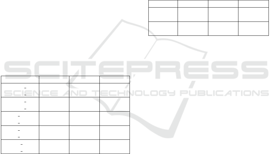
Table 1: Performance table of three sequences from Hop-
kins dataset. Comparing the algorithm with (lv) and without
(wlv) the Labeling Validation step.
Precision Recall F-score
people1 lv 0.976688 0.995086 0.985801
people1 wlv 0.069364 0.995639 0.129692
people2 lv 0.984755 0.991843 0.988286
people2 wlv 0.399106 0.990830 0.569013
cars8 lv 0.983845 0.997893 0.990819
cars8 wlv 0.635618 0.996495 0.776160
cars9 lv 0.815916 0.993595 0.896032
cars9 wlv 0.742958 0.994546 0.850537
truck2 lv 0.971608 0.983969 0.977750
truck2 wlv 0.561764 0.988119 0.716299
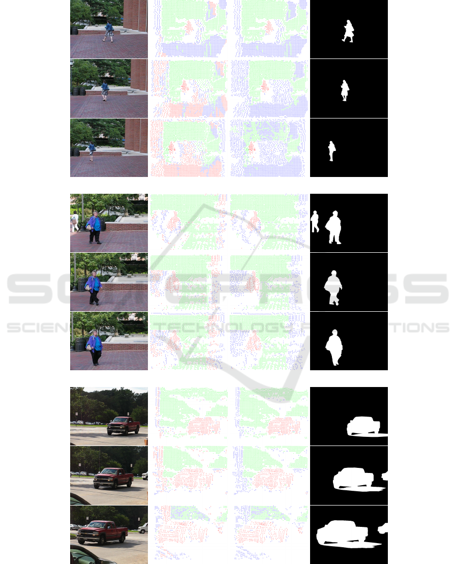
Results depicted in Figure 2 show that the ap-
proach is able to detect one or several moving ob-
jects which are rigid or non rigid. The second and
third columns of Figure 2 show the difference be-
tween moving detection without and with the Label-
ing Validation step. We observe that there are a lot
of false positive values when the Labeling Validation
is not used and there is no static point on moving ob-
jects. The precision values in the table 1 reveal that
the Labeling Validation step eliminated some false
positive values to improve the detection.
people1 and people2 sequences present high dif-
ference for the precision value with and without the
Labeling Validation. Moreover, we observed that only
the upper part of bodies are detected. It is because our
approach has to track feature points on several frames
and it is hard to track points on legs that occlude each
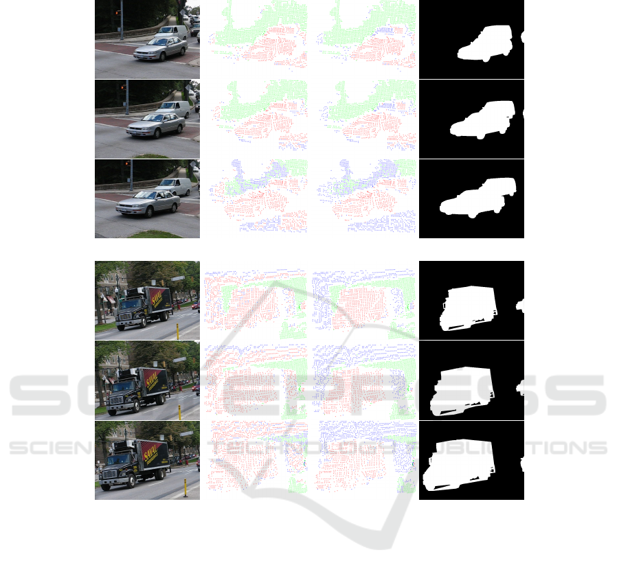
other. On the cars9 sequence, feature points at the
bottom right corner are false positive values since they
belong to the road and are labeled moving. These
points could not be corrected by the Labeling Valida-
tion step because no feature points is labeled as static
in this area. However the wrong labeling of the first
frame of 2.c is modified in the last one (there are six
frames between the first and the last frame in 2). The
precision values of cars8 and truck2 show that the La-
beling Validation step eliminated a lot of false positive
values.
Table 2: Performance table of virtual sequences. virtual1a
and virtual2a contained one moving object and virtual1b
and virtual2b had no moving object.
Precision Recall F-score
virtual1a 0.999583 0.996685 0.998132
virtual1b 1.000000 0.998092 0.999045
virtual2a 0.999214 0.999057 0.999136
virtual2b 0.973649 0.999028 0.986175
Figure 3 shows the performance of our approach
on virtual sequences. Our method does not detect
static objects as moving even if they have an optical
flow that differs from others static objects. To point
it out, we generate two sequences with the same cam-
era motion: one sequence with a moving object and
one without. The same thresholds are used in both
sequences.
The virtual1 sequence contains circular and
straight optical flow. The moving object is accurately
detected as well as the static planar surface in both vir-
tual1a and virtual1b. However, some feature points
of the planar surface on the bottom right corner of the
frame are false positive values. In this experience the
Labeling Validation step didn’t correct them because
there is no static feature point in this image region.
In the second virtual sequence virtual2, the cam-
era turns around a static object. We observe that the
static object has an optical flow different from other
static objects in the scene. In virtual2a when the
bottle moves, we observe that feature points that be-
longed to static objects are hooked to the moving ob-
ject instead of disappearing when they are occluded.
This erroneous tracking leads the Labeling Validation
step to make a mistake by correcting labels. virtual2b
contained only static objects and few points belonging
to static objects are mislabeled because of noise.
Coupled 2D and 3D Analysis for Moving Objects Detection with a Moving Camera
241

Original image
Without Labeling
Validation
With Labeling
Validation
Ground truth
(a)
(b)
(c)
Figure 2: Results of feature points labeling. Sequences of the Hopkins dataset are (a) people1, (b) people2, (c) cars8, (d) cars9
and (e) truck2. Green points are static labels, red points are moving labels and blue points are unknown labels.
VISAPP 2017 - International Conference on Computer Vision Theory and Applications
242

Original image
Without Labeling
Validation
With Labeling
Validation
Ground truth
(d)
(e)
Figure 2: Results of feature points labeling. Sequences of the Hopkins dataset are (a) people1, (b) people2, (c) cars8, (d) cars9
and (e) truck2. Green points are static labels, red points are moving labels and blue points are unknown labels. (cont.)
5 CONCLUSION AND
PERSPECTIVES
In this paper we proposed a method to detect moving
objects in the video stream of a moving camera. The
main contribution of this paper is the combination of
2D and 3D information to avoid the mislabeling of
static objects. Our approach first estimates if a fea-
ture point is moving according to 3D distances to a
rigid body. Then, the 2D optical flow corrects the es-
timation to suppress false positive labels. The rigid
body integrates feature points estimated as static over
time in order to keep the reference of 3D distances
in the field of view of the moving camera. The ad-
vantage of 3D distances to compute label estimations
is that the information is not distorted by the camera
motion. Thus, if a static object has an optical flow
which differs from others, it is still labeled as static.
Currently the user has to set thresholds of the algo-
rithm manually for each sequence. These thresholds
depend on the camera motion and the scene structure.
It would be interesting to estimate thresholds during
the initialisation step. Moreover, an additional step
could be added to the current process to propagate la-
bel information to the whole image in order to extract
silhouettes of moving objects.
Coupled 2D and 3D Analysis for Moving Objects Detection with a Moving Camera
243

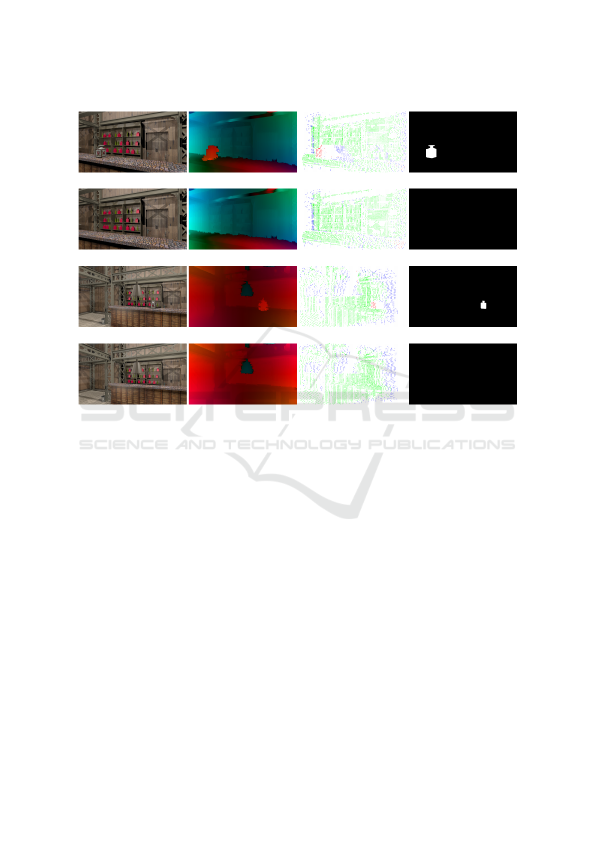
Original image Dense Optical Flow Labeling Validation Ground truth
(a)
(b)
(c)
(d)
Figure 3: Results of feature points labeling. (a) virtual1a, (b) virtual1b, (c) virtual2a, (d) virtual2b. Green points are static
labels, red points are moving labels and blue points are unknown labels.
ACKNOWLEDGEMENTS
This work is sponsored by the FUI Previz
(http://www.previz.eu). Thanks to Florian Canezin
and Julie Digne for their helpful comments and
suggestions.
REFERENCES
Brox, T. and Malik, J. (2011). Large Displacement Optical
Flow: Descriptor Matching in Variational Motion Es-
timation. IEEE Transactions on Pattern Analysis and
Machine Intelligence, 33(3):500–513.
Cui, Z., Li, A., and Jiang, K. (2014). Cooperative Mov-
ing Object Segmentation using Two Cameras based
on Background Subtraction and Image Registration.
Journal of Multimedia, 9(3):363–370.
Elqursh, A. and Elgammal, A. (2012). Online Moving
Camera Background Subtraction. In Fitzgibbon, A.,
Lazebnik, S., Perona, P., Sato, Y., and Schmid, C.,
editors, Computer Vision – ECCV 2012: 12th Euro-
pean Conference on Computer Vision, Florence, Italy,
October 7-13, 2012, Proceedings, Part VI, pages 228–
241. Springer Berlin Heidelberg.
Irani, M. and Anandan, P. (1998). A Unified Approach to
Moving Object Detection in 2D and 3D Scenes. IEEE
Transactions on Pattern Analysis and Machine Intel-
ligence, 20(6):577–589.
Jin, Y., Tao, L., Di, H., Rao, N. I., and Xu, G. (2008).
Background modeling from a free-moving camera by
Multi-Layer Homography Algorithm. In 2008 15th
IEEE International Conference on Image Processing,
pages 1572–1575.
Kim, S. W., Yun, K., Yi, K. M., Kim, S. J., and Choi, J. Y.
(2013). Detection of moving objects with a moving
camera using non-panoramic background model. Ma-
chine Vision and Applications, 24(5):1015–1028.
Narayana, M., Hanson, A., and Learned-Miller, E. (2013).
Coherent Motion Segmentation in Moving Camera
Videos Using Optical Flow Orientations. In Proceed-
ings of the 2013 IEEE International Conference on
Computer Vision, ICCV ’13, pages 1577–1584, Wash-
ington, DC, USA. IEEE Computer Society.
Nist
´
er, D. (2004). An Efficient Solution to the Five-Point
Relative Pose Problem. IEEE Trans. Pattern Anal.
Mach. Intell., 26(6):756–777.
VISAPP 2017 - International Conference on Computer Vision Theory and Applications
244

Ochs, P., Malik, J., and Brox, T. (2014). Segmentation of
Moving Objects by Long Term Video Analysis. IEEE
Transactions on Pattern Analysis and Machine Intel-
ligence, 36(6):1187–1200.
Romanoni, A., Matteucci, M., and Sorrenti, D. G. (2014).
Background subtraction by combining Temporal and
Spatio-Temporal histograms in the presence of cam-
era movement. Machine Vision and Applications,
25(6):1573–1584.
Sawhney, H. S., Guo, Y., and Kumar, R. (2000). Indepen-
dent Motion Detection in 3D Scenes. IEEE Transac-
tions on Pattern Analysis and Machine Intelligence,
22(10):1191–1199.
Sheikh, Y., Javed, O., and Kanade, T. (2009). Background
subtraction for freely moving cameras. Proceedings of
the IEEE International Conference on Computer Vi-
sion, pages 1219–1225.
Sobral, A. and Vacavant, A. (2014). A comprehensive re-
view of background subtraction algorithms evaluated
with synthetic and real videos. Computer Vision and
Image Understanding, 122:4–21.
Wang, J. Y. A. and Adelson, E. H. (1994). Representing
moving images with layers. IEEE Transactions on Im-
age Processing, 3(5):625–638.
Xue, K., Liu, Y., Ogunmakin, G., Chen, J., and Zhang,
J. (2013). Panoramic Gaussian Mixture Model and
large-scale range background substraction method for
PTZ camera-based surveillance systems. Machine Vi-
sion and Applications, 24(3):477–492.
Yi, K. M., Yun, K., Kim, S. W., Chang, H. J., and Choi,
J. Y. (2013). Detection of Moving Objects with Non-
stationary Cameras in 5.8Ms: Bringing Motion De-
tection to Your Mobile Device. In Proceedings of the
2013 IEEE Conference on Computer Vision and Pat-
tern Recognition Workshops, CVPRW ’13, pages 27–
34, Washington, DC, USA. IEEE Computer Society.
Yuan, C., Medioni, G., Kang, J., and Cohen, I. (2007). De-
tecting Motion Regions in the Presence of a Strong
Parallax from a Moving Camera by Multiview Ge-
ometric Constraints. IEEE Transactions on Pattern
Analysis and Machine Intelligence, 29(9):1627–1641.
Zamalieva, D. and Yilmaz, A. (2014). Background subtrac-
tion for the moving camera: A geometric approach.
Computer Vision and Image Understanding, 127:73–
85.
Zamalieva, D., Yilmaz, A., and Davis, J. W. (2014). A
Multi-transformational Model for Background Sub-
traction with Moving Cameras. In Fleet, D., Pajdla,
T., Schiele, B., and Tuytelaars, T., editors, Computer
VisionECCV 2014, number January 2014, pages 803–
817. Springer International Publishing, Cham.
Coupled 2D and 3D Analysis for Moving Objects Detection with a Moving Camera
245