Denoising of Noisy and Compressed Video Sequences
A. Buades and J. L. Lisani
Universitat Illes Balears, Palma de Mallorca, Spain
Keywords:
Video Denoising, Non-white Noise, Correlated Noise.
Abstract:
A novel denoising algorithm is presented for video sequences. The proposed approach takes advantage of the
self similarity and redundancy of adjacent frames. The algorithm automatically estimates a signal dependent
noise model for each level of a multi-scale pyramid. A variance stabilization transform is applied at each
scale and a novel sequence denoising algorithm is used. Experiments show that the new algorithm is able
to correctly remove highly correlated noise from dark and compressed movie sequences. Particularly, we
illustrate the performance with indoor and lowlight scenes acquired with mobile phones.
1 INTRODUCTION
Techniques for noise removal in digital images com-
prise transform thresholding, local averaging, patch
based methods and variational techniques. Nowa-
days, state of the art methods actually combine two
or three of these techniques. For example, varia-
tional and patch based techniques were combined
for both denoising and deblurring (Lou et al., 2010).
BM3D (Dabov et al., 2007) combined patch based
grouping and thresholding methods, using a 3D DCT
transform. Several methods appeared combining the
grouping of similar patches and the learning of an
adapted basis via PCA or SVD decomposition (Zhang
et al., 2010; Orchard et al., 2008). State of the art re-
sults are obtained using Gaussian models for groups
of similar patches (Lebrun et al., 2013) or adapting
the shape of the patch before learning a PCA model
(Dabov et al., 2009).
Local average methods, as the bilateral filter
(Tomasi and Manduchi, 1998), or patch based meth-
ods as NL-means (Buades et al., 2011) or BM3D
(Dabov et al., 2009) and NLBayes (Lebrun et al.,
2013) can be easily adapted to video just by extend-
ing the neighboring area to the adjacent frames. The
performance of local average methods is improved
by introducing motion compensation. These compen-
sated filters estimate explicitly the motion of the se-
quence and compensate the neighborhoods yielding
stationary data. Kervrann and Boulanger (Boulanger
et al., 2007) extended the NL-means to video by
growing adaptively the spatio-temporal neighbor-
hood. VBM4D (Maggioni et al., 2011) exploits the
mutual similarity between 3-D spatio-temporal vol-
umes constructed by tracking blocks along trajecto-
ries defined by the motion vectors.
In (Buades et al., 2016) the authors proposed to
combine optical flow estimation algorithms and patch
based methods for denoising. The algorithm was in-
spired by image fusion algorithms in the sense that
it tends to a fusion algorithm as the temporal sam-
pling of the sequence gets dense and the motion esti-
mation or global registration is able to perfectly reg-
ister the frames and no occlusions are present. As this
is an ideal scenario, the algorithm in (Buades et al.,
2016) compensates the failure of these requirements
by introducing spatiotemporal patch comparison and
denoising in an adapted PCA based transform.
It must be noted that the previous techniques are
able to deal only with uniform white noise. They are
usually tested on simulated data, by adding a Gaus-
sian noise of fixed and known variance to a noise-free
image or video. In this paper we propose a new al-
gorithm for the denoising of real (i.e. not simulated)
noisy video sequences. No noise model is assumed in
order to deal with any type of video sequence. The
noise amplitude is estimated at each level of a multi-
scale pyramid. A noise amplitude is estimated for
each color channel assuming the noise is signal de-
pendent. This is a realistic assumption since the noise
actually follows a signal dependent model at the sen-
sor (Colom et al., 2014) which is modified through
the imaging chain. The proposed algorithm removes
noise at each scale by using the white noise removal
strategy proposed in (Buades et al., 2016). Since this
strategy applies only for uniform standard deviation
150
Buades A. and Lisani J.
Denoising of Noisy and Compressed Video Sequences.
DOI: 10.5220/0006101501500157
In Proceedings of the 12th International Joint Conference on Computer Vision, Imaging and Computer Graphics Theory and Applications (VISIGRAPP 2017), pages 150-157
ISBN: 978-989-758-225-7
Copyright
c
 2017 by SCITEPRESS – Science and Technology Publications, Lda. All rights reserved

noise, a variance stabilization transform is applied at
each scale using the estimated noise amplitude values.
The whole algorithm is illustrated in Figure 1. For the
best of our knowledge, this is the first algorithm at-
tempting to join all necessary tools for denoising real
video data.
We shall proceed as follows: Section 2 summa-
rizes the method proposed in (Buades et al., 2016) for
white noise removal. Section 3 deals with the esti-
mation of noise in real image sequences. The whole
denoising chain is described in Section 4 and experi-
mental results are shown in Section 5. Finally some
conclusions are presented in Section 6.
2 IMAGE SEQUENCE WHITE
NOISE REMOVAL
In this section we briefly review the image sequence
denoising algorithm proposed in (Buades et al.,
2016). A complete description and discussion of the
algorithm can be found in the paper. The proposed
algorithm deals only with white and uniform noise.
We describe the complete algorithm for denois-
ing a frame I
k
from a sequence {I
1
,I
2
,··· ,I
N
} (Al-
gorithm 1). The same procedure is applied sequen-
tially to all the frames of the sequence. First, the op-
tical flow between I
k
and adjacent frames in a tempo-
ral neighborhood is computed and used for warping
these frames onto I
k
. If registration were accurate and
the sequence free of occlusions, a temporal average in
this static data would be optimal, even if the noise re-
duction would slowly decrease as 1/M, being M the
number of adjacent frames involved in the process.
Generally, this will not be the case, inaccuracies and
errors in the computed flow and the presence of oc-
clusions make this temporal average likely to blur the
sequence and have artifacts near occlusions. The pro-
posed approach tends to solve these limitations.
Occlusions are detected depending on the diver-
gence of the computed flow: negative divergence val-
ues indicate occlusions. Additionally, the color dif-
ference is checked after flow compensation. A large
difference indicates occlusion, or at least failure of the
color constancy assumption.
Once the neighboring frames have been warped,
the algorithm uses a 3D volumetric approach to search
for similar patches, while still 2D image patches are
used for denoising. For each patch P of the refer-
ence frame I
k
, the patch P referring to its extension
to the temporal dimension is considered, having M
times more pixels than the original one (assuming M
patches in the temporal neighborhood). Since the im-
ages have been resampled according to the estimated
flow, the data is supposed to be static. The algorithm
looks for the K extended patches closest to P . As each
extended patch contains M 2D image patches, the
group contains K · M selected patches. The Principal
Component Analysis (PCA) of these patches is com-
puted and their denoised counterparts are obtained
by thresholding of the coefficients. As proposed in
(Zhang et al., 2010), the decision of canceling a co-
efficient is not taken depending on its magnitude, but
the magnitude of the associated principal value. A
more robust thresholding is obtained by comparing
the principal values to the noise standard deviation
and canceling or maintaining the coefficients of all
the patches associated to a certain principal direction.
The whole patch is restored in order to obtain the final
estimate by aggregation.
A second iteration of the algorithm is performed
using the “oracle” strategy. Once the whole sequence
has been restored, the algorithm is re-applied on the
initial noisy sequence, but motion estimation and
patch selection are performed on the result of the first
iteration. In the same way, the PCA is computed in the
set of already denoised patches while the coefficients
of noisy patches in the computed basis are modified
by a Wiener filter strategy. In the present paper this
“oracle” strategy is not applied on the result of Algo-
rithm 1 but on the result of the whole denoising chain
(Algorithm 4).
Color images are denoised directly without the
use of any color decorrelating transform. Each color
patch is considered as a vector with three times more
components than in the single channel case. The use
of several frames makes the number of patches avail-
able much larger, relaxing the conditions on the length
of the patch vector for learning an adapted model.
This permits the use of PCA with color patches. That
is, the color decorrelation of PCA is adapted for each
group of patches, thus increasing the effectiveness of
the model.
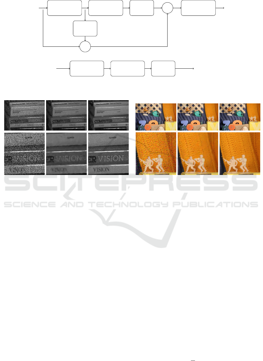
Some results of this algorithm, applied on sim-
ulated noisy sequences (with added white Gaussian
noise of known variance) are displayed in Figure 2.
This figure compares the performance of the proposed
algorithm SPTWO (Buades et al., 2016) and the state
of the art algorithm VBM4D (Maggioni et al., 2011).
Both methods are designed to deal with white uni-
form noise. We display the noisy and denoised central
frames for two image sequences of 8 frames. Both al-
gorithms are able to remove the noise, while the algo-
rithm SPTWO (Buades et al., 2016) better preserves
details and texture. The title of the book in the gray
sequence and the background texture for the color
sequence are better recovered by SPTWO. The root
mean squared errors (RMSE) between the original
Denoising of Noisy and Compressed Video Sequences
151

Downsample
Denoise
Scale 1
Upsample +
Denoise
Scale 0
Upsample
−
Input
Sequence
Denoised
Sequence
Noise Curves
Estimation
Noise Std
Stabilization
SPTWO
Input Sequence
at Scale i
Denoised Sequence
at Scale i
Figure 1: Top, illustration of the multi-scale strategy proposed for real video denoising (Algorithm 4). Only two scales are
displayed. Bottom, flow chart describing the denoising block (Algorithm 5).
Figure 2: For each of the examples, first row, from left to right: noisy frame, VBM4D, SPTWO. Second row: details of the
previous images. We display the noisy and denoised central frames of the sequence. The standard deviation for the gray
book sequence is 50, and for the color army sequence is 30. The errors for the results on the gray sequence are: VBM4D
(RMSE=6.34), SPTWO (RMSE=4.77); and for the color sequence: VBM4D (RMSE=7.35), SPTWO (RMSE=7.01). This
figure illustrates the ability of the white noise removal algorithm in (Buades et al., 2016) compared to the state of the art
VBM4D (Maggioni et al., 2011).
(noise-free) sequence and the results from VBM4D
and SPTWO, for the central frame, are displayed in
the figure caption.
3 NOISE ESTIMATION
In real video sequences (such as the ones displayed in
Figure 3) the results of the denoising algorithm pro-
posed in the previous section are far from optimal.
One reason is that in real scenes the uniform noise
model does not hold. In general, the level of noise de-
pends on the level of the signal. Moreover, even in the
case of uniform noise, the noise standard deviation is
unknown.
In the case of uniform noise, the problem can be
overcome by estimating the noise level. If the noise
is signal dependent it is also possible to estimate a
“noise curve”, that associates a noise level to each in-
tensity value of the images. Both issues are discussed
in the following subsections.
3.1 Uniform Noise
Ponomarenko et al. (Ponomarenko et al., 2007)
method estimates the noise standard deviation from
the DCT of image blocks. The DCT of each block
is computed and denoted by D
m
(i, j) where m is the
index of the block, w its size and 0 ≤ i, j < w is the
frequency pair associated to that coefficient.
The algorithm labels coefficients of the trans-
formed blocks as belonging to low (i + j < T ) or
medium/high frequencies (i + j ≥ T ), where T is a
given threshold. For each block, an (empirical) vari-
ance associated to the low-frequency coefficients of
the block m is defined V
L
m
.
The set of transformed blocks is rewritten with re-
spect to the corresponding value of V
L
m
in ascending
order. Given the list of sorted blocks {D
(m)
}, the noise
variance estimate associated with the high-frequency
coefficient at (i, j) is defined by
V
H
(i, j) =
1
K
K−1
∑
k=0

D
(k)
(i, j)

2
,
VISAPP 2017 - International Conference on Computer Vision Theory and Applications
152

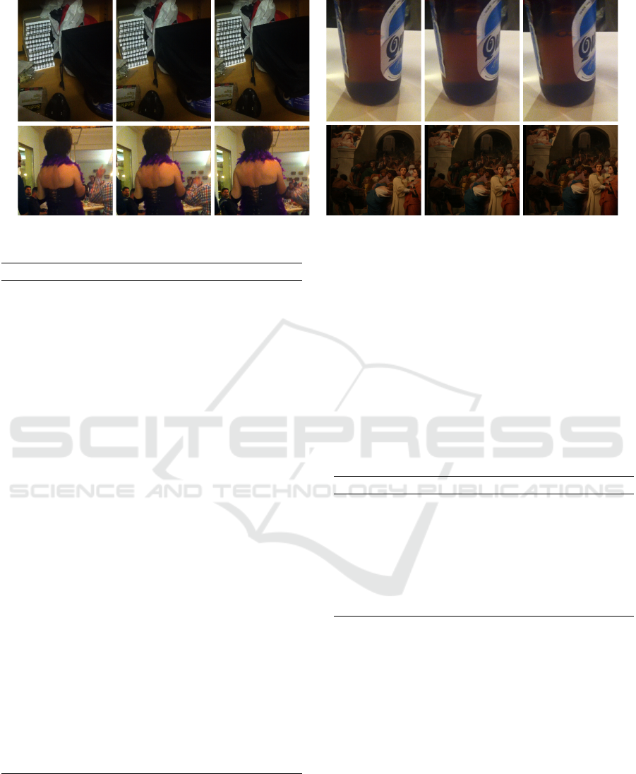
Figure 3: Some frames of the real sequences used in the experimental section of the paper.
Algorithm 1: Video Denoising (with uniform σ) (SPTWO).
Input: noisy video sequence.
Input: noise standard deviation (σ).
Output: denoised sequence.
1: for each frame I
k
in input sequence do
2: Build static sequence (S
k
) around I
k
:
3: N
k
=temporal neighborhood (M adjacent
frames)
4: Compute optical flow from I
k
to all I
j
∈ N
k
.
5: Warp all I
j
∈ N
k
using this flow.
6: for each pixel x do
7: P
x
=patches centered at x for all frames in
S
k
.
8: Remove from P
x
patches with occluded
pixels.
9: for each pixel y do
10: P
y
=patches centered at y for frames
in S
k
.
11: Remove from P
y
patches with occlu-
sions.
12: end for
13: S
K
=K closest sets P
y
to P
x
.
14: Get denoised patch
ˆ
P
x
centered at x:
15: PCA analysis of patches in S
K
16:
ˆ
P
x
=reconstruction from thresholded
coefficients in PCA basis (thresholds depend
upon σ).
17: end for
18: Get denoised frame by aggregation of de-
noised patches.
19: end for
where i + j ≥ T and K = bpMc, p < 1 is the position
of the p-quantile in the list {D
(m)
}
m∈[0,M−1]
. Note that
this empirical variance estimate is made with the list
of the K transformed blocks whose empirical variance
as measured in their low-frequencies is lowest. It is
understood that these blocks are likely to contain only
noise. Thus their high frequencies are good candi-
dates to estimate the noise. The high and low frequen-
cies are uncorrelated and since most of the energy of
the ideal image is concentrated in the low and medium
frequency coefficients (because of the sparsity of most
natural images), one can assume that V
H
(i, j) gives an
accurate estimation of the noise variance.
The final noise estimation is given by the median
of the variance estimates However, the values in the
list {V
H
(i, j)} depend on the value of the quantile K.
This is fixed to a small percentile equal to 0.5%. The
algorithm is summarized in Algorithm 2.
Algorithm 2: Ponomarenko noise estimation.
Input: W =Set of 8 × 8 image blocs (1 channel).
Output: noise level σ.
1: D = DCT (W ). 2D orthonormal DCT-II.
2: Compute V
L
=low-frequency variances of D.
3: Compute V
H
=high-frequency variances of high-
frequency blocks in D with small value in V
L
.
4: Compute σ
2
as median of variances in V
H
.
3.2 Signal Dependent Noise
In (Colom et al., 2014) it is proposed an adaptation of
the Ponomarenko noise estimation method to the case
of non-uniform noise (summarized in Algorithm 3).
For a signal dependent noise, a “noise curve” must
be established. This noise curve associates with each
image value U(x,y) an estimation of the standard de-
viation of the noise . Thus, for each block in the im-
age its mean is computed and gives an estimation of a
value in U.
The means of these blocks are classified into a dis-
joint union of variable intervals or bins, in such a way
that each interval contains a large enough number of
elements. That is, the gray level range is not divided
Denoising of Noisy and Compressed Video Sequences
153

into uniform length intervals, but these intervals are
adapted to the image itself. This way, if the image is
dark, most part of the intervals will be of short length
and belonging to dark values while none or very few
bins will be in the lighter part of the gray level range.
These measurements allow for the construction of a
list of block standard deviations whose corresponding
means belong to the given bin.
Algorithm 3: Signal-dependent noise estimation.
Input: noisy video sequence.
Output: noise curves (for each color channel).
1: Extract all 8 ×8 (overlapping) blocks from all the
frames in input sequence.
2: for each color channel do
3: Compute average value of each block.
4: Classify blocks in bins according to average
value. Adapt number of bins such that every bin
contains at least 42000 blocks.
5: for each bin i do
6: Get set of points (λ
i
,σ
i
) where
σ
i
=Ponomarenko(bins
i
) (Algorithm 2) and
λ
i
=average value bin i.
7: end for
8: Interpolate (λ
i
,σ
i
) values.
9: Filter noise curve.
10: end for
Therefore, it is possible to apply the noise esti-
mation algorithm described in the previous section to
each set of blocks associated with a given bin. In this
way, an estimation of the noise for the intensities in-
side the limits of the bin is obtained.
This noise estimation algorithm will be applied at
each level of the multi-scale pyramid. Figure 4 dis-
plays the noise curves estimated for some of the video
sequences used in this paper and three scales, the orig-
inal fine scale and two more. In order to compute
these curves we have used a pyramid with a subsam-
pling of factor two at each scale, obtained by simple
averaging of four pixels. We do not apply any convo-
lution since we want our algorithm to work also with
white noise. If the noise at the finest scale is white,
this ensures that it stays white during the whole pyra-
mid and the noise standard deviation is divided by
two at each scale. This is not the case for the curves
displayed in the figure since the initial noise was not
white.
We must emphasize that these curves are not ex-
actly the same ones that will be obtained during the
denoising process explained in the next section. Dur-
ing the denoising process, at a certain scale, lower
ones are already denoised, and therefore the images
for which the noise curves are estimated are differ-
ent from the ones in this experiment. The figure dis-
plays the noise pairs (u
i
,σ(u
i
)) for each channel and
the interpolated ones by using a polynomial of degree
2. The polynomial fits well with the estimated noise
pairs. These curves are quite similar to the ones pro-
posed by (Liu et al., 2008) even if the methods are
quite different since this latter algorithm estimates ac-
tually a noise model taking into account the demo-
saicking, tone curve and color corrections applied by
the camera.
4 PROPOSED ALGORITHM
The noise being nearly white at the CFA sensor gets
correlated by the demosaicking process. The rest
of the imaging chain consisting mainly in color and
gamma correction enhances the noise in dark parts of
the image leading to colored spots of several pixels.
The size of these spots depends on the demosaicking
method applied. In order to remove such noise we
use a multi-scale strategy aiming at denoising each of
these spots at the correct scale where they look like
white noise.
4.1 Multi-scale
The proposed algorithm decomposes the image in a
multi-scale pyramid and, at each level, the noise is es-
timated, the variance stabilized and the noise removed
by the white noise removal algorithm detailed in Sec-
tion 2. Once the lowest scale is denoised, the result
is up-sampled and the details added back. Down-
sampling at each scale is performed by averaging
groups of four pixels (factor 2 downsampling) while
up-sampling is done using cubic splines interpolation.
The procedure is repeated until the finest scale is at-
tained. The multi-scale strategy is illustrated in Fig-
ure 1.
4.2 Noise Standard Deviation
Stabilization
As commented in the previous section, the denoising
algorithm proposed in Section 2 (Algorithm 1) fails to
denoise a real video sequence due to the fact that, in
general, the noise level is not uniform but depends on
the intensity level of the images. However, the noise
curve relating intensity values and noise levels can be
learnt from the video sequence (Algorithm 3) and the
original video sequence can be manipulated in order
to achieve a uniform noise distribution with arbitrary
noise level. This manipulation is known as the
Anscombe transform (described in the next para-
VISAPP 2017 - International Conference on Computer Vision Theory and Applications
154

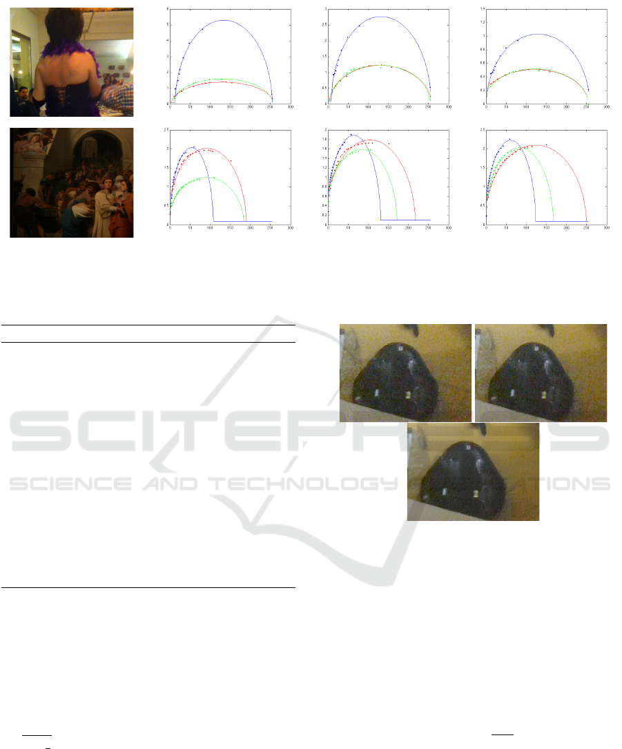
Figure 4: Display of noise curves for different image sequences and three scales. The algorithm is applied at each scale
obtained from the previous one by subsampling of factor two, obtained by agglomeration of four pixels. The noise pairs
(u
i
,σ(u
i
)) obtained by the algorithm proposed in Section 3.2 are displayed for each channel and interpolated by using a
polynomial of degree 2. The polynomial fits well with the estimated noise pairs.
Algorithm 4: Multi-scale Blind Video Denoising.
Input: noisy video sequence ˜u
0
.
Input: number of scales N.
Output: denoised sequence ˆu
0
.
1: for s = 1···N − 1 do
2: Noisy sequence (scale s): ˜u
s
=
downsample( ˜u
s−1
)
3: Details: d
s−1
= ˜u
s−1
− upsample( ˜u
s
)
4: end for
5: Set ¯u
N−1
= ˜u
N−1
.
6: for s = N − 1···1 do
7: Denoise: ˆu
s
= denoise( ¯u
s
) (with Algo-
rithm 5).
8: Add details: ¯u
s−1
= upsample( ˆu
s
) + d
s−1
9: end for
10: Set ˆu
0
= ¯u
0
.
graph) and it is an invertible transform. It is there-
fore possible to apply Algorithm 1 to denoise the
transformed sequence and to obtain the final denoised
video using the inverse Anscombe transform. The
method is summarized in Algorithm 5.
The Anscombe Transform. We usually refer to the
Anscombe transform as to the transformation f (u) =
2
q
u +
3
8
which is known to stabilize the variance
of a Poisson noise model. However, any signal de-
pendent additive noise can be stabilized by a simple
transform. Let v = u + g(u)n be the noisy signal, we
search for a function f such that f (v) has uniform
standard deviation. When the noise is small com-
pared to the signal we can apply the decomposition
f (v) = f (u) + f
0
(u)g(u)n. Forcing the noise term to
Figure 5: Comparison of the application of the chain with
a single scale (top-right) or three scales (bottom) as used
by our method. The original image is displayed in the
top-left corner of the figure. The images have been en-
hanced (Drago et al., 2003) in order to better illustrate the
differences between the two methods. The single scale al-
gorithm actually removes noise but only noise values of
slightly more than one pixel but not large spots. Large col-
ored spots are removed only by the multi-scale algorithm,
which removes them at the scale for which they become al-
most white noise.
be constant, f
0
(u)g(u) = c, and integrating we obtain
f (u) =
Z
u
0
cdt
g(t)
.
When a linear variance noise model is taken, this
transformation gives back the known Anscombe
transform.
We apply this transformation with the curve ob-
tained at each scale in order to stabilize the noise vari-
ance. The inverse transform is applied back after de-
noising to get the original range.
Denoising of Noisy and Compressed Video Sequences
155

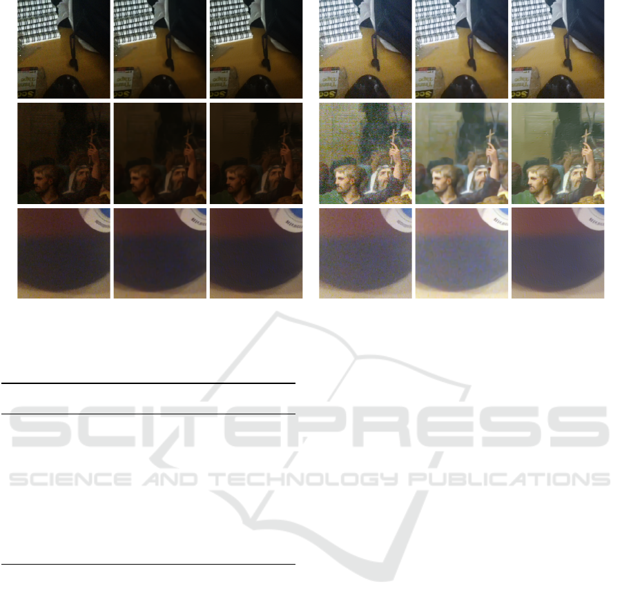
Figure 6: Denoising examples. From left to right the first three columns display: excerpt from the central frame of the original
sequence, VBM4D result, result of the proposed chain. The noise standard deviation used as a parameter of the VBM4D
algorithm is 15 for each sequence. The same images are displayed in the last three columns after enhancement (Drago et al.,
2003) for better visualization of the differences.
Algorithm 5: Video Denoising (with signal-dependent un-
known noise).
Input: noisy video sequence.
Output: denoised sequence.
1: Compute noise curves for the input sequence (Al-
gorithm 3).
2: Apply Anscombe transform to the input se-
quence, based on the previous noise curves.
3: Denoise video (Algorithm 1).
4: Apply inverse Anscombe transform to obtain the
final denoised sequence.
4.3 Denoising Algorithm and the
Second Iteration Question
The denoising algorithm in (Buades et al., 2016) has
originally two steps as explained in Section 2. In the
second step the already denoised image is used in or-
der to compute the patch distances and learn the PCA
model.
A straightforward extension of the method to the
multi-scale video algorithm would apply the two steps
for each particular image at each scale. Instead, we
apply only the first step at each scale and after the im-
age sequence or video has been completely denoised,
a second step is applied. The second step takes as in-
put the completely filtered sequence, and for the de-
noising of a particular image and scale, the already
denoised image at that scale is used for selecting the
similar patches and learn the PCA model.
5 EXPERIMENTATION
In this section we illustrate the performance of the
proposed method and the importance of each stage.
All experiments use exactly the same parameters
which mainly are the number of scales, the window
size and the filtering parameter. We used three scales,
a 5 ×5 window and a filtering parameter equal to 4.0σ
at each scale. The denoising stage is applied after the
variance stabilization transform for which the stan-
dard deviation curve is estimated automatically. We
used the proposed method in Algorithm 3 with 10 bins
and the curve was approximated by a polynomial of
degree 2.
We first illustrate the need of a multi scale algo-
rithm. Figure 5 compares the application of the chain
with a single scale or three scales as proposed. The
denoised images are afterwards enhanced (with the
tone mapping algorithm described in (Drago et al.,
2003)) in order to better illustrate the differences
between the two methods. The single scale algo-
rithm actually removes noise but only noise values of
slightly more than one pixel but not large spots. Large
colored spots are removed only by the multi-scale al-
gorithm, which removes them at the scale for which
they become almost white noise.
Figure 6 compares our method with state of the
VISAPP 2017 - International Conference on Computer Vision Theory and Applications
156

art algorithm VBM4D (Maggioni et al., 2011). It
must be remarked that this algorithm is not designed
for real image noise but for the denoising of white
and uniform noise. Moreover, an estimation of the
noise variance must be provided. In our exam-
ples we tested with different noise variances (σ =
{10,15,20,25,30}). We display the best results for
each video sequence. The figure also displays the im-
ages after enhancement. This enhancement permits
a better visualization of the noise removal but is not
part of the proposed chain. These examples show that
the proposed denoising method outperforms state of
the art techniques and illustrates the need of such a
complex chain with multi-scale and signal dependent
noise estimation and stabilization.
One short movie displaying the results of the de-
noising chain can be found in the supplementary ma-
terials accompanying this paper.
6 CONCLUSIONS
We have proposed a denoising algorithm for real
video comprising all stages, multi-scale, noise esti-
mation and denoising. The proposed algorithm has
shown to effectively remove highly correlated noise
from dark and compressed movie sequences with
weak signal-to-noise ratio.
ACKNOWLEDGEMENTS
The authors gratefully acknowledge support by grant
TIN2014-53772-R. The second author was also sup-
ported by grant TIN2014-58662-R.
REFERENCES
Boulanger, J., Kervrann, C., and Bouthemy, P. (2007).
Space-time adaptation for patch-based image se-
quence restoration. IEEE Trans. PAMI, 29(6):1096–
1102.
Buades, A., Coll, B., and Morel, J. (2011). Self-similarity-
based image denoising. Communications of the ACM,
54(5):109–117.
Buades, A., Lisani, J., and Miladinovi
´
c, M. (2016). Patch
Based Video Denoising with Optical Flow Estimation.
IEEE Transactions on Image Processing, 25(6).
Colom, M., Buades, A., and Morel, J.-M. (2014). Nonpara-
metric noise estimation method for raw images. JOSA
A, 31(4):863–871.
Dabov, K., Foi, A., Katkovnik, V., and Egiazarian, K.
(2007). Image denoising by sparse 3D transform-
domain collaborative filtering. IEEE Transactions on
image processing, 16:2007.
Dabov, K., Foi, A., Katkovnik, V., Egiazarian, K., et al.
(2009). Bm3d image denoising with shape-adaptive
principal component analysis. Proc. of the Workshop
on Signal Processing with Adaptive Sparse Structured
Representations, Saint-Malo, France.
Drago, F., Myszkowski, K., Annen, T., and Chiba, N.
(2003). Adaptive logarithmic mapping for display-
ing high contrast scenes. In Proceedings of EURO-
GRAPHICS, volume 22.
Lebrun, M., Buades, A., and Morel, J.-M. (2013). A nonlo-
cal bayesian image denoising algorithm. SIAM Jour-
nal on Imaging Sciences, 6(3):1665–1688.
Liu, C., Szeliski, R., Kang, S., Zitnick, C., and Freeman, W.
(2008). Automatic estimation and removal of noise
from a single image. IEEE transactions on pattern
analysis and machine intelligence, 30(2):299–314.
Lou, Y., Zhang, X., Osher, S., and Bertozzi, A. (2010). Im-
age recovery via nonlocal operators. Journal of Scien-
tific Computing, 42(2):185–197.
Maggioni, M., Boracchi, G., Foi, A., and Egiazarian, K.
(2011). Video denoising using separable 4D nonlocal
spatiotemporal transforms. In IS&T/SPIE Electronic
Imaging, pages 787003–787003. International Society
for Optics and Photonics.
Orchard, J., Ebrahimi, M., and Wong, A. (2008). Effi-
cient Non-Local-Means Denoising using the SVD. In
Proceedings of The IEEE International Conference on
Image Processing.
Ponomarenko, N. N., Lukin, V. V., Zriakhov, M. S., Kaarna,
A., and Astola, J. T. (2007). An automatic approach
to lossy compression of AVIRIS images. IEEE Inter-
national Geoscience and Remote Sensing Symposium.
Tomasi, C. and Manduchi, R. (1998). Bilateral filtering for
gray and color images. In Computer Vision, 1998.
Sixth International Conference on, pages 839–846.
Zhang, L., Dong, W., Zhang, D., and Shi, G. (2010). Two-
stage image denoising by principal component anal-
ysis with local pixel grouping. Pattern Recognition,
43(4):1531–1549.
Denoising of Noisy and Compressed Video Sequences
157