Selective Maintenance for Failure-prone Multi-state Systems When the
Durations of Missions and Scheduled Breaks Are Stochastic
A. Khatab
1
and E. H. Aghezzaf
2
1
Laboratory of Industrial Engineering, Production and Maintenance (LGIPM),
National School of Engineering, Metz, France
2
Department of Industrial Systems Engineering and Product Design,
Faculty of Engineering and Architecture, Ghent University, Ghent-Zwijnaard, Belgium
Keywords:
Selective Maintenance, Reliability, Imperfect Maintenance, Stochastic Optimization.
Abstract:
This paper addresses the selective maintenance optimization problem for a multi-component and multi-state
system (MSS). The system performs several missions with breaks between each two consecutive missions.
At the end of a mission, the reliability of the system is defined as the probability that the system satisfies the
required demand level during the next mission. This probability is evaluated using the z-transform method. To
improve the system’s reliability, its components are maintained during breaks. To each component, a list of
maintenance actions is available from minimal repair to overhaul through imperfect maintenance actions. Du-
rations of missions and breaks are considered not constant but rather stochastic. These durations are therefore
modeled as random variables with appropriate probability distributions. The selective maintenance optimiza-
tion problem proposed is modeled as a non-linear and stochastic program. The fundamental constructs and
the relevant parameters of this decision-making problem are solely investigated and discussed. An illustra-
tive example is provided to demonstrate the added value of solving this selective maintenance problem as a
stochastic optimization program.
1 INTRODUCTION
Selective maintenance is dedicated especially to
multi-component systems operating an alternate se-
quence of missions and scheduled breaks. To suc-
cessfully execute the next mission, maintenance activ-
ities are performed on the system components during
the scheduled breaks. However, due the limited dura-
tion of a scheduled break, in addition to the possible
budget and maintenance resources constraints, only a
set of components may indeed be selected for main-
tenance. To meet the minimum predetermined per-
formance level required to operate the next mission,
it is therefore mandatory to select an optimal set of
components to maintain as well as the type of mainte-
nance actions to be performed on these components.
Selective maintenance was first introduced by
(Rice et al., 1998) and applied for a series-parallel
system where each subsystem is composed of inde-
pendent and identical components. The lifetime of
each system’s component is assumed to follow an ex-
ponential distribution and the replacement of failed
component is the only one maintenance alternative to
improve system’s reliability. To overcome the draw-
back hypothesis of independent and identically dis-
tributed components in (Rice et al., 1998), (Cassady
et al., 2001b) proposed a more generalized selective
maintenance modeling framework for systems whose
reliability block diagram may be a combination of se-
ries, parallel and bridge structures. (Cassady et al.,
2001a) considered the selective maintenance prob-
lem for a series-parallel system where components’
lifetimes are Weibull distributed. Three maintenance
actions are then considered, namely the minimal re-
pair, the corrective replacement of failed components
and the preventive replacement of functioning com-
ponents. To solve the resulting optimization problem,
an exhaustive enumeration method is used. In (Ra-
jagopalan and Cassady, 2006), the authors proposed
four improved enumeration procedures to reduce the
computational time in (Cassady et al., 2001b). To
deal with selective maintenance problem for large
sized systems, (Khatab et al., 2007) proposed two
heuristic-based methods. The authors in (Lust et al.,
2009) proposed also an exact method based on the
branch-and-bound procedure and a Tabu search algo-
rithm. More recently, imperfect maintenance actions
are considered in the selective maintenance setting.
210
Khatab, A. and Aghezzaf, E.
Selective Maintenance for Failure-prone Multi-state Systems When the Durations of Missions and Scheduled Breaks Are Stochastic.
DOI: 10.5220/0005823802100217
In Proceedings of 5th the International Conference on Operations Research and Enterprise Systems (ICORES 2016), pages 210-217
ISBN: 978-989-758-171-7
Copyright
c
 2020 by SCITEPRESS – Science and Technology Publications, Lda. All rights reserved

(Zhu et al., 2011) considered the age reduction coef-
ficient approach of (Malik, 1979) to model imperfect
preventive maintenance. (Panday et al., 2013) also
studied the selective maintenance problem for binary
systems under imperfect PM. They considered, the
hybrid hazard rate model introduced by (Lin et al.,
2000) to model imperfect maintenance actions. The
authors in (Djelloul et al., 2015) considered selective
maintenance problem in the case the system operates
missions of random duration.
The selective maintenance studied in the above
mentioned works merely rely on binary state systems
having only two operating states, namely function-
ing and failure states. However, many industrial sys-
tems are designed to operate their tasks according to
a range of performance levels varying from perfect
functioning to complete failure. Such systems are
known as multi-state systems (MSS). Dealing with
selective maintenance of MSS, only few works ap-
peared in the literature. The first work is reported
in (Chen et al., 1999). Each system’s component as
well as the system itself may be in one of the (K + 1)
possible states. Replacement of failed components
is the only available maintenance option. A mainte-
nance optimization problem is then derived to min-
imize the total maintenance cost while providing a
given required system reliability level for the next
mission. To solve this problem, a procedure based on
the short path method is proposed. In (Liu and Huang,
2010), the authors studied the selective maintenance
problem for a MSS where components are character-
ized by two operating states (functioning and failure
states) while the system performs several states with
different output performance levels. Several mainte-
nance options are also considered from minimal re-
pair to replacement through imperfect maintenance.
A genetic algorithm is used to solve the resulting se-
lective maintenance optimization problem. To over-
come the restrictive hypothesis of binary components
in (Liu and Huang, 2010), (Pandey et al., 2013) stud-
ied selective maintenance for a series-parallel MSS
where components are characterized by more than
one performance level (i.e. multi-state components).
The transition rates between states of a component
are assumed constants, i.e. components are mod-
eled as continuous-time Markov chain. In (Khatab
and Ait-Kadi, 2008), the authors generalized the se-
lective maintenance optimization problem to consider
more than one mission. To improve the reliability of
the system, preventive maintenance actions are per-
formed during breaks. The selective maintenance
problem consists on finding an optimal sequence of
maintenance actions the cost of which minimizes the
total maintenance cost while providing the desired
system reliability level for each mission. The result-
ing optimization problem is solved using the extended
great deluge algorithm.
Dealing with the MSS selective maintenance
problem, all the above mentioned papers assumed
that the duration of the break as well as that of the
next mission are both known and constant. However,
this assumption may no longer be valid in many real-
world situations where it is usually difficult to eval-
uate the exact duration of a mission. Indeed, such
duration may unfortunately be impacted by the occur-
rence of random events which lead the system either
to abort the mission or at most to continue operating
the mission but with more additional time. Similarly,
the occurrence of random events may conduct the de-
cision maker to shorten or even to extend the break
duration. As a consequence, it is more realistic and
practical to consider that mission as well as break du-
rations are not precisely known but rather random and
should therefore be governed by appropriate probabil-
ity distributions.
The present paper addresses the selective main-
tenance problem for a MSS systems when the du-
ration of the next mission and that of the break are
stochastic and modeled as random variables. Right
after each mission, the system becomes available for
maintenance during a limited duration of the break,
to meet the required reliability level for the execution
of the next mission. Due to the limited maintenance
resources, not all components are likely to be main-
tained. The selective maintenance decision problem
to be solved consists first in selecting a subset of com-
ponents and then choosing the level of maintenance
to be performed on each of the selected components.
The objective function may consist of maximizing the
successful completion of the next mission while tak-
ing into account maintenance budget and time allotted
to the break, or of minimizing the total maintenance
cost subject to the required reliability level and the
time allotted to the break, or of minimizing the to-
tal maintenance time subject to the required reliability
level and the maintenance budget. The present paper
considers the second objective function. The stochas-
tic selective maintenance problem is then formulated
and solved.
The remainder of this paper is organized as fol-
lows. Section 2 describes the investigated system
and defines its reliability. Section 2 shows how the
z−transform is used to estimate MSS reliability. Sec-
tion 3 presents the imperfect maintenance model and
defines time and cost for each maintenance action.
Section 4 discusses the reliability computation to op-
erate missions of random durations. The stochastic
selective maintenance optimization model is devel-
Selective Maintenance for Failure-prone Multi-state Systems When the Durations of Missions and Scheduled Breaks Are Stochastic
211

oped and discussed in Section 5. A numerical exam-
ple is provided to illustrate the benefit of considering
stochastic durations of missions and breaks. Finally,
some conclusions are drawn in Section 6.
2 SYSTEM DESCRIPTION AND
RELIABILITY COMPUTATION
The selective maintenance problem addressed in the
present work concerns a multi-state system (MSS) S
composed of n failure-prone components. Each com-
ponent C
i
(i = 1,... ,n) is characterized by two per-
formance rates g
i1
= 0 and g
i2
6= 0. The later is the
nominal output performance when component C
i
is
functioning, while the former corresponds to the out-
put performance when C
i
fails. In this paper, the per-
formance of a system’s component is defined by its
productivity or capacity. The entire system is there-
fore characterized by a range of K = 2
n
performance
levels from complete failure up to perfect functioning.
Let G
k
be the output performance level of the k
th
sys-
tem’s state and Pr{G(t) = G
k
} = q
k
(t)(k = 1,. .. ,K)
with G(t) being the output performance of the system
at time t. Then, the output performance distribution
(OPD) of the system can be completely determined
by the following two sets G and q:
G = {G
k
: 1 6 k 6 K}, and (1)
q = {q
k
(t) : 1 6 k 6 K}. (2)
The reliability R(t,W ) of the MSS is defined as its
ability to satisfy the required performance level (de-
mand) W at a given time t. Since G(t) represents the
output performance of the system at time t, this relia-
bility is then defined as (Xue and Yang, 1995):
R(t,W ) = Pr{G(t) > W }. (3)
According to Equations (1) and (2), the MSS reliabil-
ity is equivalently defined as the probability that the
system resides during the time interval [0,t] in states
where the output performance level is at least equal to
the required demand W . Therefore, the MSS reliabil-
ity is given as:
R(t,W ) = Pr{G(t) > W }
=
∑
G
k
>W
q
k
(t). (4)
In the present work, MSS reliability computation is
performed on the basis of the universal z-transform
techniques developed in (Ushakov, 1986). In the lit-
erature, the universal z-transform is also called univer-
sal moment generating function (UMGF) and denoted
as u-function. For more details, te reader may refers
to (Levitin and Lisnianski, 2001; Lisnianski and Lev-
itin, 2003; Levitin, 2005). The UMGF corresponding
to the MSS S is given by the polynomial U(t,z) such
that:
U(t,z) =
K
∑
k=1
q
k
(t) ·z
G
k
. (5)
From the above equation, the MSS reliability can then
be computed as:
R(t,W ) = Pr{G(t) > W }
=
K
∑
k=1
q
k
(t) ·Φ(z
G
k
−W
), (6)
where Φ is a function defined as:
Φ(z
G
k
−W
) =

1 if G
k
> W,
0 otherwise.
To evaluate the MSS reliability, two basic operators
are defined. The UMGF corresponding to the entire
system reliability is then obtained by using simple al-
gebraic operations on individual UMGF of systems’
components. These operators allow to take into ac-
count how components are connected in series or in
parallel. To illustrate, let us consider the simple case
of a MSS composed of two components C
1
and C
2
characterized, respectively, by the UMGF u
1
(t,z) and
u
2
(t,z) such that:
u
1
(t,z) = q
11
(t) ·z
g
11
+ q
12
(t) ·z
g
12
= q
11
(t) ·z
0
+ q
12
(t) ·z
g
12
, and (7)
u
2
(t,z) = q
21
(t) ·z
g
21
+ q
22
(t) ·z
g
22
= q
21
(t) ·z
0
+ q
22
(t) ·z
g
22
. (8)
In the above equations, parameters g
i1
= 0 and g
i2
rep-
resent the output performance levels of component C
i
,
while q
i1
(t) and q
i2
(t) are the instantaneous probabil-
ities corresponding, respectively, to the output perfor-
mance levels g
i1
and g
i2
. In this paper, performance of
a components and that of the system itself is defined
by productivity. Therefore, if components C
1
and C
2
are connected in parallel, the resulting MSS produc-
tivity is the sum of its components’ productivity. In
this case, the UMGF of the MSS is given as:
U(t,z) =
2
∑
i=1
2
∑
j=1
q
1i
(t) ·q
2 j
(t) ·z
g
1i
+g
2 j
. (9)
However, the total productivity of components C
1
and
C
2
connected in series corresponds to the minimum
of all components capacities. In this case, the UMGF
U(t,z) corresponding to the MSS is given as:
U(t,z) =
2
∑
i=1
2
∑
j=1
q
1i
(t) ·q
2 j
(t) ·z
min(g
1i
,g
2 j
)
. (10)
ICORES 2016 - 5th International Conference on Operations Research and Enterprise Systems
212

3 IMPERFECT MAINTENANCE
MODEL AND RELATED COST
AND TIME
To perform maintenance activities, a list of L
i
main-
tenance options (levels) {1, .. ., l
i
,. ..,L
i
} is available
for each component C
i
. Among these maintenance
options, there are two particular values l
i
= 1 and
l
i
= L
i
. The former corresponds to the minimal re-
pair maintenance action that when performed brings
the component to an as bad as old conditions, while
the later corresponds to the overhaul after which the
component becomes as as good as new. Values of
l
i
where 1 < l
i
< L
i
represent imperfect maintenance
actions such that when performed they bring the com-
ponent’s condition between the as good as new and
as bad as old conditions. In the present paper, the age
reduction coefficient of Malik (Malik, 1979) is used
to model the imperfect maintenance options. Accord-
ing to this model, when an imperfect maintenance ac-
tion is performed on a component it reduces its age
from, say t, to θ ×t where θ is the age reduction coef-
ficient (0 ≤ θ ≤ 1). Accordingly, the system becomes
as good as new (overhaul)if its age is reset to zero
(θ = 0) while it becomes as bad as old (minimal re-
pair) if the age reduction coefficient θ = 1.
The maintenance cost MC(l
i
) induced by a main-
tenance action of level l
i
when performed on com-
ponent C
i
is a preventive maintenance cost MC
p
(l
i
)
if C
i
is functioning at the end of the current mis-
sion, or a corrective maintenance cost MC
c
(l
i
) if C
i
is failed at the end of the current mission. Simi-
larly, the maintenance time MT (l
i
) consumed by a
maintenance action of level l
i
executed on compo-
nent C
i
is equal to MT
p
(l
i
) if C
i
is still functioning
at the end of the current mission, or MT
c
(l
i
) oth-
erwise. The particular values of maintenance cost
MC(l
i
) and maintenance time MC(l
i
) are defined for
l
i
= 1 (minimal repair) and l
i
= L
i
(overhaul). For
a failed component MC
c
(1) = MRC
i
, MC
c
(L
i
) =
OC
c
i
, MT
c
(1) = MRT
i
, and MT
c
(L
i
) = OT
c
i
. In the
case where the component is functioning at the end
of the current mission, the cost MC
p
(L
i
) and time
MT
p
(L
i
) induced by preventive overhauling compo-
nent C
i
are defined, respectively, as MC
p
(L
i
) = OC
p
i
and MT
p
(L
i
) = OT
p
i
. Maintenance cost MC
p
(1) and
maintenance time MT
p
(1) are not eligible since min-
imal repair is assumed to be admissible as a mainte-
nance option only for a failed component.
4 PROBABILITY OF NEXT
MISSION SUCCESS
Let us assume that the system have just finished a mis-
sion and then, turned off during the scheduled break
of finite length and becomes available for possible
maintenance activities. The system is thereafter used
to execute the next mission of a given duration. When
the system is set for maintenance, a component can be
either in a functioning state or in a failed state. Hence,
two state variables X
i
and Y
i
are used to describe the
status of component C
i
, respectively, at the beginning
and at the end of a mission:
Y
i
=



1, if C
i
is functioning at the end of
the current mission,
0, otherwise.
(11)
X
i
=



1, if C
i
is functioning at the beginning
of the next mission,
0, otherwise.
(12)
In what follows we let A
i
be the age of the compo-
nent at the beginning of the next mission and B
i
be
the age of C
i
at the end of the current mission. Fur-
thermore, duration D of the scheduled break is a ran-
dom variable governed by a probability density func-
tion (pdf) f
D
(t) and a cumulative distribution func-
tion (cdf) F
D
(t). The duration of the next mission is
also stochastic and represented by a random variable
O whose pdf and cdf are denoted by f
O
(t) and F
O
(t),
respectively.
According to the age reduction imperfect PM
model, if a maintenance action with an eligible level l
i
is performed on component C
i
at the end of the current
mission, the effective age A
i
of C
i
at the beginning of
the next mission becomes then:
A
i
= θ
l
i
·B
i
. (13)
Let R
c
i
be the conditional probability that component
C
i
successfully operates the next mission given that its
initial age is A
i
at the beginning of the next mission.
If T
i
denotes the random variable of the lifetime of
component C
i
, then the conditional reliability R
c
i
is
evaluated as:
R
c
i
= Pr(T
i
> A
i
+ O
|
T
i
>A
i
). (14)
Taking into account Equation (13), and the fact that
O is a random variable governed by the cdf F
O
(t) de-
fined on the support [O
min
,O
max
], then the conditional
reliability R
c
i
is evaluated to:
R
c
i
=
R
O
max
O
min
R
i
(θ
l
i
·B
i
+ u) ·dF
O
(t)
R
i
(θ
l
i
·B
i
)
(15)
In the above equation R
i
(t) refers to the uncondi-
tional survival function of component C
i
. According
Selective Maintenance for Failure-prone Multi-state Systems When the Durations of Missions and Scheduled Breaks Are Stochastic
213

to Equation (15), the UMGF u
1
(O,z) corresponding
to component C
i
is written as:
u
1
(O,z) = (1 −R
c
i
) ·(1 −X
i
) ·z
g
i1
+ R
c
i
·X
i
·z
g
i2
(16)
Let us denote q
i1
(O) = (1 −R
c
i
) · (1 −X
i
) and
q
i2
(O) = R
c
i
·X
i
. Let us also denote W
0
the required
demand level to be satisfied during the next mission
with stochastic duration O. Using results of Section
2, the UMGF U(O,z) of the entire system is evaluated
as:
U(O,z) =
K
∑
k=1
q
k
(O) ·z
G
k
. (17)
where q
k
(O) stands for the probability that the system
resides in state k(k = 1,. .. ,K) at the end of the next
mission, and G
k
is the system’s output performance
in that state. Following the development of Section 2,
the probability R(O,W
0
) that the system successfully
operate the next mission is given as:
R(O,W
0
) =
K
∑
k=1
q
k
(O) ·Φ(z
G
k
−W
0
). (18)
5 THE STOCHASTIC SELECTIVE
MAINTENANCE
OPTIMIZATION PROBLEM
Assume that the system has just operated the current
mission and system’s components may undergo main-
tenance activities. However, not all components may
possibly be maintained due to the limitation on both
maintenance budget and time. Consequently, a selec-
tive maintenance problem must be solved. The ob-
jective consists then on minimizing the total main-
tenance cost taking into account, on one hand, the
required minimal system’s reliability to successfully
completing the next mission, and the limited duration
of the break, on the other hand. The probability of
completing the next mission is obtained from the re-
liability R(O,W
0
) given by Equation (18). To evalu-
ate the total cost induced by maintenance actions and
the corresponding total time consumed from the break
duration, we define the following decision variable
s
i
(l
i
):
s
i
(l
i
) =



1, if C
i
is selected for maintenance and
maintenance level l
i
is performed,
0, otherwise.
(19)
The total cost of maintenance during the break is de-
noted by T MC and computed as:
T MC = PMC +CMC, (20)
where PMC and CMC denote the total cost induced
by, respectively, preventive and corrective mainte-
nance actions performed during the break. The to-
tal cost of preventive maintenance actions is evaluated
as:
PMC =
n
∑
i=1
L
i
∑
l
i
=2
MC
p
(l
i
) ·Y
i
·s
i
(l
i
), (21)
where a PM action of level l
i
> 1 is allowed to be per-
formed on component C
i
only if C
i
is in working state
at the end of the current mission, i.e. Y
i
= 1. By anal-
ogy, the total cost induced by corrective maintenance
actions is evaluated as:
CMC =
n
∑
i=1
L
i
∑
l
i
=1
MC
c
(l
i
) ·(1 −Y
i
) ·s
i
(l
i
), (22)
where (1 −Y
i
) states that corrective maintenance ac-
tions are available only for failed components.
The total time required to perform maintenance ac-
tions during the break is also composed of preven-
tive and corrective maintenance times denoted, re-
spectively, by PMT and CMT . These quantities are
evaluated to:
PMT =
n
∑
i=1
L
i
∑
l
i
=2
MT
p
(l
i
) ·Y
i
·s
i
(l
i
), (23)
CMT =
n
∑
i=1
L
i
∑
l
i
=1
MT
c
(l
i
) ·(1 −Y
i
) ·s
i
(l
i
). (24)
Hence, the total time spent in maintenance during the
break is denoted by T MT and computed as:
T MT = PMT +CMT. (25)
The stochastic selective maintenance optimization
problem is then formulated as follows:
Min




n
∑
i=1
L
i
∑
l
i
=1
MC
c
(l
i
) ·(1 −Y
i
) ·s
i
(l
i
)
+
n
∑
i=1
L
i
∑
l
i
=2
MC
p
(l
i
) ·Y
i
·s
i
(l
i
)




(26)
Subject to:
R(O,W
0
) ≥ R
0
,
(27)
Pr(D ≥ T MT ) ≥ τ
s
,
(28)
L
i
∑
l
i
=1
(1−Y
i
) ·s
i
(l
i
) +
L
i
∑
l
i
=2
Y
i
·s
i
(l
i
) ≤ 1,
(29)
s
i
(1) ≤ 1 −Y
i
,
(30)
X
i
= Y
i
+
L
i
∑
l
i
=1
(1−Y
i
) ·s
i
(l
i
),
(31)
A
i
= [θ
l
i
·s
i
(l
i
) + (1 −s
i
(l
i
))] ·B
i
,
(32)
s
i
(l
i
) ∈ {0, 1}; i = 1, .. ., n; l
i
= 1,... ,L
i
.
ICORES 2016 - 5th International Conference on Operations Research and Enterprise Systems
214

In the above optimization model, Equations (27)
and (28) are, respectively,the required reliability level
and the maintenance time constraints. The constraint
(28) is the newly introduced constraint requiring par-
ticular treatment. In fact, the probability of executing
a selective maintenance plan should at least be equal
to a required service ratio τ
s
. This constraint ensures
with the probability at least equal to τ
s
that the se-
lected components will be maintained each with the
corresponding selected maintenance level. The risk
corresponding to the inability to perform a selected
maintenance plan is then evaluated to 1 −τ
s
. This re-
sults from the fact that the duration of the break is
considered stochastic rather than constant. For each
component C
i
, Equations (29) states that only one
maintenance level can be selected if the component is
to be maintained. The constraint (30) states that mini-
mal repair is eligible only on a failed component. The
constraint (31) allows to update the operating state of
components. For a given system’s configuration, this
stochastic optimization problem can be solved using
the usual stochastic optimization techniques. The fol-
lowing section presents an illustrative examples and
discusses how the stochasticity of the mission and
break durations impact the maintenance level selec-
tion decisions. In this experiment, durations and costs
are respectively given in time and monetary units.
6 NUMERICAL EXAMPLE
This experiment investigates the selective main-
tenance problem for a series-parallel MSS whith
stochastic durations of missions and breaks. The sys-
tem is composed of two series subsystems. The first
subsystem is composed of 3 parallel components C
i
(i = 1, 2,3), and the second also contains 3 compo-
nents C
i
(i = 4,5, 6) arranged in parallel. The failure
time of the system’s component C
i
follows a Weibull
distribution whose shape and scale parameters are re-
spectively given by β
i
and η
i
(i = 1, .. ., n). Values of
these parameters are shown in Table (1). This table
shows also components’ performance rates g
i2
, the
value of B
i
corresponding to the age of components
C
i
at the end of the current mission, in addition to the
value of the state variables Y
i
corresponding to the its
operating state (functioning or failed). According to
this table, only components C
1
and C
4
survived the
current mission (Y
1
= Y
4
= 1) while the other compo-
nents are in failed state.
A same list of L
i
= 6 (i = 1,. .. ,6) possible main-
tenance levels is available for all system’s compo-
nents. Age reduction coefficients corresponding to
these maintenance levels are given in Table (2). Cor-
Table 1: Components’ parameters.
C
i j
) β
i
η
i
g
i2
Y
i
B
i
C
1
1.5 75 55 1 35
C
2
2.4 114 80 0 24
C
3
1.6 84 120 0 45
C
4
2.4 102 70 1 36
C
5
2.5 78 95 0 44
C
6
2.0 84 80 0 28
Table 2: Maintenance levels and their respective age reduc-
tion coefficient values.
l
i
1 2 3 4 5 6
θ
l
i
1 0.7 0.5 0.3 0.2 0
Table 3: Minimal repair and corrective maintenance costs.
C
i
l
i
C
1
C
2
C
3
C
4
C
5
C
6
1 5 6 6 6 5 5
2 2.81 0.32 3.48 1.88 5.29 1.74
3 5.88 1.73 6.28 4.41 7.99 4.58
4 9.56 5.25 9.27 7.73 10.49 8.65
5 11.59 8.15 10.81 9.65 11.69 11.14
6 16 17 14 14 14 17
rective maintenance costs and times are given, respec-
tively, in Tables (3) and (4), while preventive mainte-
nance costs and times are shown in Tables (5) and (6),
respectively.
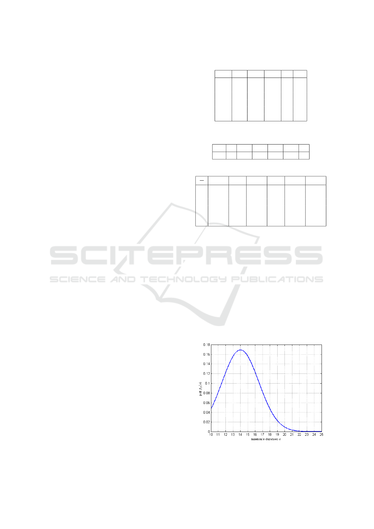
For the analysis below, we assume that the dura-
tion of the break is deterministic and fixed to D = 10,
while the duration O of the next mission is stochas-
tic and governed by a truncated normal distribution
N (14,2.5) on the support [10,25] (see Figure 1).
We also set the required minimum level of the sys-
tem’s reliability R
0
to execute the next mission to
R
0
= 70% with a required demand W
0
= 150. If
no maintenance is performed on the systems’ com-
ponents, the probability of the system successfully
completing the next mission is null. Indeed, only
Figure 1: The pdf corresponding to the duration of the next
mission.
Selective Maintenance for Failure-prone Multi-state Systems When the Durations of Missions and Scheduled Breaks Are Stochastic
215

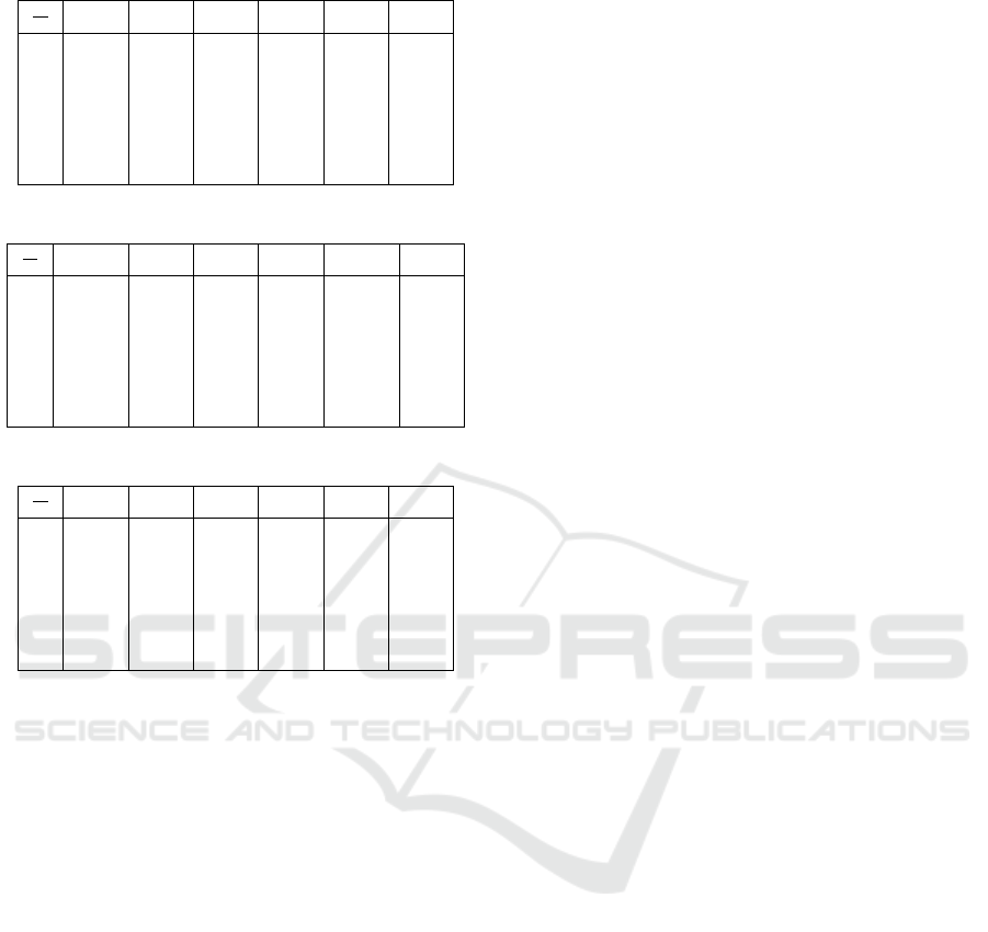
Table 4: Minimal repair and corrective maintenance times.
C
i
l
i
C
1
C
2
C
3
C
4
C
5
C
6
1 2 2 3 3 3 2
2 0.7 0.08 1.24 0.67 1.89 0.41
3 1.47 0.41 2.24 1.57 2.85 1.08
4 2.39 1.23 3.31 2.76 3.75 2.04
5 2.9 1.92 3.86 3.45 4.17 2.62
6 4 4 5 5 5 4
Table 5: Preventive maintenance costs.
C
i
l
i
C
1
C
2
C
3
C
4
C
5
C
6
1 − − − − − −
2 2.46 0.28 2.98 1.61 4.53 1.43
3 5.14 1.53 5.38 3.78 6.85 3.77
4 8.36 4.63 7.94 6.62 8.99 7.13
5 10.14 7.19 9.27 8.27 10.02 9.18
6 14 15 12 12 12 14
Table 6: Preventive maintenance times.
C
i
l
i
C
1
C
2
C
3
C
4
C
5
C
6
1 − − − − − −
2 0.35 0.04 0.25 0.13 0.38 0.2
3 0.73 0.2 0.4 0.31 0.57 0.54
4 1.19 0.62 0.66 0.55 0.75 1.02
5 1.45 0.96 0.77 0.69 0.83 1.31
6 2 2 1 1 1 2
components C
1
and C
4
are functionning at the end
of the current mission mission. Therefore, the total
out put performance of the the system is evaluated to
min(g
12
,g
42
) = min(55, 70) = 55 which is less than
the required minimum demand level W
0
. To improve
this reliability, the selective maintenance problem is
therefore solved.
Given the required minimum demand W
0
with the
reliability level R
0
, and the limited time D of the
break, if the selective maintenance problem in solved
by assuming the deterministic duration of the next
mission (i.e. the next mission duration is set to 14.12
which is the average value of O), in this case the
optimal selective maintenance plan suggested is as
follows. Components C
1
and C
4
are selected to un-
dergo preventive maintenance actions of levels, re-
spectively, 6 and 2,i.e. a preventive overhaul is per-
formed on C
1
and an imperfect maintenance is exe-
cuted on C
2
. Furthermore, components C
3
and C
6
are
selected to undergo corrective maintenance actions of
levels, respectively, 5 and 2. This maintenance plan
induces a total cost T MC = 30.86 and requires a total
time T MT = 5.95. The resulting system’s reliability
is evaluated to 70.20%. Applying this maintenance
plan in the case where the duration of the next mis-
sion is stochastic leads to a system’s reliability equal
to 61.95% which is indeed less than the required min-
imum reliability level R
0
. In the stochastic case, this
selective maintenance plan is unable to allow the sys-
tem’s reliability to reach the required minimum level
for the next mission. Thus, if for some reason, the
mission duration is extended, there will be then a high
risk of not completing the mission with the required
reliability level. However, if this same selective main-
tenance problem is solved by considering the dura-
tion of the next mission to be stochastic, the follow-
ing selective maintenance plan is obtained according
to which components C
1
and C
4
are selected to un-
dergo preventive maintenance actions of levels, re-
spectively, 6 and 3. In addition, components C
3
and
C
5
are selected to receive corrective maintenance of
levels 5 and 4. The resulting system’s reliability is
evaluated to 70.41%. The total cost induced by this
selective maintenance plan is T MC = 40.29 and the
corresponding total maintenance time is T MT = 8.02.
Let us now consider the additional constraint rep-
resented by the stochastic limited break duration D.
This duration is also modeled as a random variable
with pdf and cdf, respectively, denoted by f
D
(d) and
F
D
(d). They are defined on a support [D
min
,D
max
]
meaning that the break takes a duration d which
lies between D
min
and D
max
. In the present exam-
ple, we assume that D follows a uniform distribution
U(6, 14); its corresponding average value is E(D) =
10. It follows that the probability to successfully
performing the selective maintenance plan is given
by Pr(T MT ≤ D) = 1 −F
D
(T MT ) and evaluated to
74.75%. Accordingly, the selective maintenance plan
is then a feasible solution of the stochastic selective
optimization problem only if the service ratio level
τ
s
is fixed to a value less than or equal to 74.75%
(τ
s
≤ 74.75%).
7 CONCLUSION
This paper addressed the selective maintenance op-
timization problem for multi-component and multi-
state system. For each component of the system, a
list of maintenance actions is available from minimal
repair to overhaul through imperfect maintenance ac-
tions. Each maintenance actions is characterized by
a reliability improvement level. The system performs
several missions separated by scheduled breaks dur-
ing which maintenance activity can takes place. Du-
rations of both breaks and missions are considered as
random variables governed by an appropriate proba-
bility distributions. These distributions are integrated
in the selective maintenance problem resulting in a
non-linear stochastic optimization program. A nu-
ICORES 2016 - 5th International Conference on Operations Research and Enterprise Systems
216

merical example is studeied to demonstrate how the
stochasticity of missionss durations impacts the se-
lective maintenance decisions.
REFERENCES
Cassady, C. R., Murdock, W. P., and Pohl, E. A. (2001a).
Selective maintenance for support equipement involv-
ing multiple maintenance actions. European Journal
of Operational Research, 129:252–258.
Cassady, C. R., Pohl, E. A., and Murdock, W. P. (2001b).
Selective maintenance modeling for industrial sys-
tems. Journal of Quality in Maintenance Engineering,
7(2):104–117.
Chen, C., Mend, M. Q.-H., and Zuo, M. J. (1999). Selective
maintenance optimization for multi-state systems. In
In Proc. of the IEEE Canadian Conference on Electri-
cal and Computer Engineering, Edmonton, Canada.
Djelloul, I., Khatab, A., Aghezzaf, E.-H., and Sari, Z.
(2015). Optimal selective maintenance policy for
series-parallel systems operating missions of random
durations. In International confrence on Computers &
Industrial Engineering (CIE 45), Metz, France.
Khatab, A. and Ait-Kadi, D. (2008). Selective maintenance
policy multi-state series parallel systems. In 4th Inter-
national Conference on Advances in Mechanical En-
gineering and Mechanics, Sousse, Tunisia.
Khatab, A., Ait-Kadi, D., and Nourelfath, M. (2007).
Heuristic-based methods for solving the selective
maintenance problem for series-prallel systems. In In-
ternational Conference on Industrial Engineering and
Systems Management, Beijing, China.
Levitin, G. (2005). Universal generating function in relia-
bility analysis and optimization. Springer-Verlag.
Levitin, G. and Lisnianski, A. (2001). A new approach to
solving problems of multi-state system reliability op-
timization. Quality and Reliability Engineering inter-
national, 17:93–104.
Lin, D., Zuo, M. J., and Yam, R. C. M. (2000). General
sequential imperfect preventive maintenance mod-
els. International Journal of Reliability, Quality and
Safety Engineering, 7(3):253–266.
Lisnianski, A. and Levitin, G. (2003). Multi-state systems
reliability: Assesment, optimization and applications.
World Scientific.
Liu, Y. and Huang, H.-Z. (2010). Optimal selective main-
tenance strategy for multi-state systems under imper-
fect maintenance. IEEE Transactions on Reliability,
59(2):356–367.
Lust, T., Roux, O., and Riane, F. (2009). Exact and heuristic
methods for the selective maintenance problem. Eu-
ropean Journal of Operational Research, 197:1166–
1177.
Malik, M. (1979). Reliable preventive maintenance
scheduling. AIIE transactions, 11(3):221–228.
Panday, M., Zuo, M. J., Moghaddass, R., and Tiwari, M. K.
(2013). Selective maintenance for binary systems un-
der imperfect repair. Reliability Engineering and Sys-
tem Safety, 113:42–51.
Pandey, M., Zuo, M., and Moghaddass, R. (2013). Selec-
tive maintenance modeling for multistate system with
multistate components under imperfect maintenance.
IIE Transcations, 45:1221–1234.
Rajagopalan, R. and Cassady, C. R. (2006). An improved
selective maintenance solution approach. Journal of
Quality in Maintenance Engineering, 12(2):172–185.
Rice, W. F., Cassady, C. R., and Nachlas, J. (1998). Op-
timal maintenance plans under limited maintenance
time. In Proceedings of Industrial Engineering Con-
ference, Banff, BC, Canada.
Ushakov, I. (1986). Universal generating function. So-
viet Journal of Computing System Science, 24(5):118–
129.
Xue, J. and Yang, K. (1995). Dynamic reliability analysis
of coherent multi-state systems. IEEE Transactions
on Reliability, 44(4):683–688.
Zhu, H., Liu, F., Shao, X., Liu, Q., and Deng, Y. (2011).
A cost-based selective maintenance decision-making
method for machining line. Quality and Reliability
Engineering International, 27:191–201.
Selective Maintenance for Failure-prone Multi-state Systems When the Durations of Missions and Scheduled Breaks Are Stochastic
217