Application of the Hamiltonian Formulation
to Nonlinear Light-envelope Propagations
Guo Liang
1,2
, Qi Guo
1,∗
and Zhanmei Ren
1
1
Guangdong Provincial Key Laboratory of Nanophotonic Functional Materials and Devices, South China Normal
University, Guangzhou 510631, P. R. China
2
School of Physics and Electrical Information, Shangqiu Normal University, Shangqiu 476000, P. R. China
Keywords:
Canonical Equations of Hamilton, the Nonlocal Nonlinear Schr¨odinger Equation, Optical Solitons.
Abstract:
A new approach, which is based on the new canonical equations of Hamilton found by us recently, is presented
to analytically obtain the approximate solution of the nonlocal nonlinear Schr¨odinger equation (NNLSE). The
approximate analytical soliton solution of the NNLSE can be obtained, and the stability of the soliton can
be analytically analysed in the simple way as well, all of which are consistent with the results published
earlier. For the single light-envelope propagated in nonlocal nonlinear media modeled by the NNLSE, the
Hamiltonian of the system can be constructed, which is the sum of the generalized kinetic energy and the
generalized potential. The extreme point of the generalized potential corresponds to the soliton solution of the
NNLSE. The soliton is stable when the generalized potential has the minimum, and unstable otherwise.
1 INTRODUCTION
The propagations of the (1+D)-dimensional light-
envelopes in nonlinear media have been studied ex-
tensively for a few decades (Agrawal, 2001; As-
santo, 2012b; Trillo and Torruellas, 2001; Kivshar
and Agrawal, 2003; Stegeman and Segev, 1999; Chen
et al., 2012; Malomed et al., 2005), which are gov-
erned by the following dimensionless model (Chen
et al., 2015):
i
∂ϕ
∂z
+ ∇
2
⊥
ϕ+ ∆nϕ = 0, (1)
where ϕ(r,z) is the complex amplitude envelop,
∆n(r,z) is the light-induced nonlinear refractive in-
dex, z is the longitudinal coordinate, r is the D-
dimensional transverse coordinate vector with D be-
ing the positive integer, and ∇
⊥
is the D-dimensional
differential operator vector of the transverse coordi-
nates. Generally, ∆n(r,z) can be phenomenologically
expressed as the convolution between the response
function R(r) of the media and the modulus square
of the light-envelope ϕ(r,z) for the bulk media with
the nonlocal nonlinearity (Chen et al., 2015; Assanto,
2012a; Snyder and Mitchell, 1997; Krolikowski et al.,
2001)
∆n(r,z) =
Z
∞
−∞
R(r−r
′
)|ϕ(r
′
,z)|
2
d
D
r
′
. (2)
According to the relative scale of the characteristic
length of the response function R and the scale in the
transverse dimension occupied by the light-envelope
ϕ, the degree of nonlocality can be divided into four
categories(Chen et al., 2015; Krolikowski et al., 2001;
Assanto, 2012a): local, weakly nonlocal, generally
nonlocal, and strongly nonlocal, and locality is the
case when the response function R is the Dirac delta
function. In the local case, Eq.(1) is reduced to
i
∂ϕ
∂z
+ ∇
2
⊥
ϕ+ |ϕ|
2
ϕ = 0. (3)
Eq. (1) together with the nonlocal nonlinearity (2) is
called as the nonlocal nonlinear Schr¨odinger equation
(NNLSE) (Chen et al., 2015; Assanto, 2012a; Kro-
likowski et al., 2001), while its special case, Eq. (3),
is the well-known nonlinear Schr¨odinger equation
(NLSE) (Kivshar and Agrawal, 2003; Agrawal, 2001;
Trillo and Torruellas, 2001).
The NNLSE (with its special case NLSE) can
describe the nonlinear propagations of the optical
beams (Assanto, 2012b; Trillo and Torruellas, 2001;
Stegeman and Segev, 1999; Chen et al., 2012; Kivshar
and Agrawal, 2003), the optical pulses (Agrawal,
2001; Kivshar and Agrawal, 2003) and the optical
pulsed beams (Kivshar and Agrawal, 2003; Malomed
et al., 2005). The second term of the NNLSE ac-
counts for the diffraction for the first case where r

is the spatial transverse coordinate, the group veloc-
ity dispersion (GVD) for the second case where r is
the time coordinate, and both the diffraction and the
GVD for the last case where r is both the spatial trans-
verse coordinate and the time coordinate, while the
third term (the nonlinear term) describes the compres-
sion of the light-envelopes for all cases. Specifically,
when D = 1, the NNLSE can model the propaga-
tion of the optical beam (Snyder and Mitchell, 1997;
Krolikowski et al., 2001) in the self-focusing nonlin-
ear planar waveguide, and can also model the prop-
agation of the optical pulse (Agrawal, 2001) in the
self-focusing nonlinear waveguide if the carrier fre-
quency is in the anomalous GVD regime or in the
self-defocusing nonlinear waveguide when its carrier
frequency is in the normal GVD regime. The (1+1)-
dimensional NNLSE has the spatial (or temporal)
bright optical soliton solution (Kivshar and Agrawal,
2003). When D = 2, the NNLSE can only describe
the propagation of the optical beam in the nonlinear
bulk media. The bright spatial optical soliton can
exist stably for the nonlocal case (Assanto, 2012a),
but for the local case the strong self-focusing of a
two dimensional beam will lead to the catastrophic
phenomenon (Kivshar and Pelinovsky, 2000). When
D = 3, the NNLSE can describe the propagation of
the optical pulsed beams. Like the case of D = 2, the
self trapped optical pulsed beam propagating in the
local nonlinear media will lead to the spatiotemporal
collapse (Silberberg, 1990), which can be arrested by
the nonlocal nonlinearity (Malomed et al., 2005). But
when D > 3, the NNLSE is just a phenomenological
model, the counterpart of which can not be found in
physics. It’s important to note that(Chen et al., 2015)
the response function R is symmetric for the spatial
nonlocality, but is asymmetric for the temporal non-
locality due to the causality (Hong et al., 2015).
As the special case of the NNLSE, the NLSE (3)
can be solved exactly using inverse-scattering tech-
nique (Zakharov and Shabat, 1971; Zakharov and
Shabat, 1973) when D = 1. But for the general
case, a closed-form solution of NNLSE (1) cannot
been found except for the strongly nonlocal limit,
where the NNLSE can be simplified to the (linear)
Snyder-Mitchell model for the spatial nonlocality and
an exact Gaussian-shaped stationary solution known
as accessible soliton was found (Snyder and Mitchell,
1997). Approximately analytical solutions can be ob-
tained by various of perturbation methods, such as the
perturbation approach based on the inverse scattering
transform (Karpman and Maslov, 1977), the adiabatic
perturbation approach (Kivshar and Malomed, 1989),
the method of moments (Maimistov, 1993), and the
most widely used one is variational method (Ander-
son, 1983; Guo et al., 2006; Chen et al., 2013; Wolf,
2002). It was claimed without proof that the varia-
tional method can only be applied in nonlocal cases
where the response function is symmetric (Steffensen
et al., 2012). And for the case of the response function
without even symmetry, the method of moments can
work well. Another new approach is presented here,
and we apply the canonical equations of Hamilton to
study the nonlinear light-envelope propagations. By
taking this approach, the approximate analytical soli-
ton solution of the NNLSE is obtained. Furthermore,
the stability of solutions can be analysed analytically
in a simple way as well, but it can not be done by the
variational approach.
2 CANONICAL EQUATIONS OF
HAMILTON FOR THE NNLSE
As has been known (Anderson, 1983), the variational
approach to find the approximately analytical solution
of the NNLSE is based on the Euler-Lagrange equa-
tions. In the classical mechanics, however, there exist
two theory frameworks: the Lagrangian formulation
(the Euler-Lagrange equations) and the Hamiltonian
formulation (canonical equations of Hamilton). The
two methods are parallel, and no one is particularly
superior to the another for the direct solution of me-
chanical problems (Goldstein et al., 2001). The new
approach presented in this paper to analytically ob-
tain the approximate solution of the NNLSE is based
on the new canonical equations of Hamilton (CEH)
found by us recently (Liang et al., 2013). For the sake
of the systematicness and the readability of this pa-
per, the key points about the new CEH are outlined
here in this section, although the detail can be found
in Ref (Liang et al., 2013).
We firstly define two different systems of mathe-
matical physics (Liang et al., 2013): the second-order
differential system (SODS) and the first-order differ-
ential system (FODS). The SODS is defined as the
system described by the partial differential equation
that contains the second-order partial derivative with
respect to the evolution coordinate, while the FODS is
defined as the system described by the partial differ-
ential equation that contains only the first-order par-
tial derivativewith respect to the evolution coordinate.
The Newton’s second law of motion and the NNLSE
are the exemplary SODS and FODS, where the evo-
lution coordinates are the time coordinate t and the
propagation coordinate z, respectively. The conven-
tional CEH (Goldstein et al., 2001)is established on
the basis of the Newton’s second law of motion.

˙q
i
=
∂H
∂p
i
, (4)
− ˙p
i
=
∂H
∂q
i
, (5)
The dot above the variable in Eqs. (4) and (5) ( ˙q
i
and
˙p
i
) indicates the derivative with respect to the evolu-
tion coordinate (here the evolution coordinate is the
time t), q
i
and p
i
are said to be the generalized coor-
dinate and the generalized momentum, and H is the
Hamiltonian. The CEH (4) and (5) can be extended
to the continuous system as (Goldstein et al., 2001)
˙q
s
=
δh
δp
s
, (6)
− ˙p
s
=
δh
δq
s
, (7)
with s = 1,··· ,N representing the components of the
quantity of the continuous system (Goldstein et al.,
2001),
δh
δq
s
=
∂h
∂q
s
−
∂
∂x
∂h
∂q
s,x
and
δh
δp
s
=
∂h
∂p
s
−
∂
∂x
∂h
∂p
s,x
de-
note the functional derivatives of h with respect to q
s
and p
s
with q
s,x
=
∂q
s
∂x
and p
s,x
=
∂p
s
∂x
, and h is the
Hamiltonian density of the continuous system.
We have shown that the FODS can not be ex-
pressed by the conventional CEH, and we have re-
constructed a set of new CEH through the following
procedure.
For the first-order differential system of the con-
tinuous systems, the Lagrangian density must be the
linear function of the generalized velocities, and ex-
pressed as
l =
N
∑
s=1
R
s
(q
s
) ˙q
s
+ Q(q
s
,q
s,x
), (8)
where R
s
is not the function of a set of q
s,x
with q
s,x
=
∂q
s
/∂x. Consequently, the generalized momentum p
s
,
which is obtained by the definition p
s
= ∂l/∂ ˙q
s
as
p
s
= R
s
(q
s
),(s = 1, ···, N), (9)
is only a function of q
s
. There are 2N variables,
q
s
and p
s
, in Eqs. (9). The number of Eqs. (9)
is N, which also means there exist N constraints
between q
s
and p
s
. So the degree of freedom of
the system given by Eqs. (9) is N. Without loss
of generality, we take q
1
,··· ,q
ν
and p
1
,··· , p
µ
as
the independent variables, where ν + µ = N. The
remaining generalized coordinates and generalized
momenta can be expressed with these independent
variables as q
α
= q
α
(q
1
,··· ,q
ν
, p
1
,··· , p
µ
)(α = ν +
1,··· ,N), and p
β
= p
β
(q
1
,··· ,q
ν
, p
1
,··· , p
µ
)(β =
µ+ 1,··· ,N). The Hamiltonian density h for the con-
tinuous system is obtained by the Legendre transfor-
mation as h =
∑
N
s=1
˙q
s
p
s
−l, where the Hamiltonian
density h is a function of ν generalized coordinates,
q
1
,··· ,q
ν
, and µ generalized momenta, p
1
,··· , p
µ
.
We can obtain the new CEH consisting of N equations
as
δh
δq
λ
=
N
∑
s=1

˙q
s
∂p
s
∂q
λ
− ˙p
s
∂q
s
∂q
λ

+
N
∑
α=ν+1
∂
∂x
∂h
∂q
α,x
∂q
α
∂q
λ
, (10)
δh
δp
η
=
N
∑
s=1

˙q
s
∂p
s
∂p
η
− ˙p
s
∂q
s
∂p
η

+
N
∑
α=ν+1
∂
∂x
∂h
∂q
α,x
∂q
α
∂p
η
, (11)
where λ = 1, ··· , ν, η = 1,··· ,µ, and ν + µ = N. The
CEH (10) and (11) can be easily extended to the dis-
crete system, which can be expressed as
∂H
∂q
λ
=
N
∑
s=1

˙q
s
∂p
s
∂q
λ
− ˙p
s
∂q
s
∂q
λ

, (12)
∂H
∂p
η
=
N
∑
s=1

˙q
s
∂p
s
∂p
η
− ˙p
s
∂q
s
∂p
η

, (13)
where λ = 1,··· ,ν, η = 1,··· ,µ, ν+ µ = N, the gen-
eralized momenta are defined as
p
i
=
∂L
∂ ˙q
i
, (14)
with L =
R
∞
−∞
ld
D
r being the Lagrangian, and the
Hamiltonian is obtained by Legendre transformation
as
H =
n
∑
i=1
˙q
i
p
i
−L. (15)
For the SODS, all the generalized coordinates and the
generalized momenta are independent, the new CEH
(12) and (13) are automatically reduced to the con-
ventional CEH (4) and (5).
We have shown that the FODS can only be ex-
pressed by the new CEH, but do not by the conven-
tional CEH, while the SODS can be done by both the
new and the conventional CEHs. We have also shown
that the NLSE can be expressed by the new CEH in a
consistent way if the propagation coordinate z in the
NLSE is considered to be the evolution coordinate.
3 APPLICATION OF THE NEW
CEH TO LIGHT-ENVELOPE
PROPAGATIONS
Different from the case of the NLSE, the Hamilto-
nian density of the NNLSE contains the convolution
between the response function R(r) and the modulus
square of the light-envelope ϕ(r,z). Following the
procedure in Sec. 2, it can be easily proved that the
NNLSE can also be expressed with the new CEH in a
consistent way if the propagation coordinate z in the
model is considered to be the evolution coordinate.

Based on the new CEH, we now introduce a new ap-
proach to deal with the nonlinear light-envelopeprop-
agations.
We assume the trial solution of the form as
ϕ(r,z) = q
A
(z)exp

−
r
2
q
2
w
(z)

exp

iq
c
(z)r
2
+ iq
θ
(z)

,
(16)
where q
A
,q
θ
are the amplitude and phase of the com-
plex amplitude of the light-envelope, respectively, q
w
is the width of the light-envelope,q
c
is the phase-front
curvature, and they all vary with the propagation dis-
tance (the evolution coordinate) z. The response func-
tion of materials is assumed as
R(r) =
1
(
√
πw
m
)
D
exp

−
r
2
w
2
m

. (17)
Inserting the trial solution (16) and the response func-
tion (17) into the Lagrangian density
l =
i
2

ϕ
∗
∂ϕ
∂z
−ϕ
∂ϕ
∗
∂z

−|∇
⊥
ϕ|
2
+
1
2
|ϕ(r,z)|
2
∆n(r,z), (18)
and performing the integration L =
R
∞
−∞
ld
D
r we
obtain
L = −2
−2−D
π
D/2
q
2
A
q
−2+D
w
(w
2
m
+ q
2
w
)
−D/2
[−2q
2
A
q
2+D
w
+2
D/2
(w
2
m
+ q
2
w
)
D/2
(4D+ 4Dq
2
c
q
4
w
+ Dq
4
w
˙q
c
+ 4q
2
w
˙q
θ
)], (19)
which is a function of generalized coordinates,
q
A
,q
w
,q
c
and generalized velocities, ˙q
c
, ˙q
θ
(The dot
above the variable indicates the derivative with re-
spect to the evolution coordinate z), but not an ex-
plicit function of the evolution coordinate z. Eq. (16)
can be understood as a “coordinate transformation”.
Through such a transformation (of course, this is not
a real coordinate transformation in the rigorous sense
in mathematics), the coordinate system consist of a set
of generalized coordinates ϕ and ϕ∗ is transformed to
that consist of another set of generalized coordinates
q
A
, q
w
, q
c
, and q
θ
, and the Lagrangian density ex-
pressed by Eq. (18) in the continuous system is trans-
ferred to the Lagrangian expressed by Eq. (19) in the
discrete system at the same time via the integration
L =
R
∞
−∞
ld
D
r.
Then the generalized momenta can be obtained by
definition (14) as follows
p
A
= p
w
= 0, (20)
p
c
= −2
−2−
D
2
Dπ
D/2
q
2
A
q
2+D
w
, (21)
p
θ
= −

π
2

D/2
q
2
A
q
D
w
. (22)
The Hamiltonian of the system then can be deter-
mined by Legendre transformation (15)
H = 2
−1−D
π
D/2
q
2
A
q
−2+D
w
(w
2
m
+ q
2
w
)
−D/2
[−q
2
A
q
2+D
w
+2
1+
D
2
D(w
2
m
+ q
2
w
)
D/2
(1+ q
2
c
q
4
w
)], (23)
and can be proved to be a constant, i.e.
˙
H = 0.
There are four generalized coordinates and four
generalized momenta in the four equations (20), (21)
and (22). So the degree of freedom of the set of
equations (20), (21) and (22) is four. Without loss
of generality, we take q
c
,q
θ
, p
c
and p
θ
as the in-
dependent variables. By solving Eqs.(21) and (22),
the generalized coordinates q
A
and q
w
can be ex-
pressed by generalized momenta p
c
and p
θ
as q
A
=
(−p
θ
)
1/2
[Dp
θ
/(2πp
c
)]
D/4
and q
w
= [4p
c
/(Dp
θ
)]
1/2
,
and inserting this result into the Hamiltonian (23)
yields
H = −
D
2
p
2
θ
+ 16p
2
c
q
2
c
4p
c
−
1
2
π
−D/2
(
4p
c
Dp
θ
+ w
2
m
)
−D/2
. (24)
By use of the canonical equations of Hamilton
(12) and (13) in the case that µ = ν = 2 and n = 4 be-
cause there are only two independent generalized co-
ordinates and two independent generalized momenta,
we can obtain the following four equations
˙q
c
=
D
2
p
2
θ
4p
2
c
−4q
2
c
+
Dπ
−D/2
p
2
θ
(
4p
c
Dp
θ
+ w
2
m
)
−D/2
4p
c
+ Dp
θ
w
2
m
, (25)
˙q
θ
= −
(4+ D)π
−D/2
p
c
p
θ
(
4p
c
Dp
θ
+ w
2
m
)
−D/2
4p
c
+ Dp
θ
w
2
m
−
D
2
p
θ
2p
c
−
Dπ
−D/2
p
2
θ
w
2
m
(
4p
c
Dp
θ
+ w
2
m
)
−D/2
4p
c
+ Dp
θ
w
2
m
, (26)
˙p
c
= 8p
c
q
c
, (27)
˙p
θ
= 0. (28)
It can be found that the generalized coordinate q
θ
is not contained in the Hamiltonian (24), then q
θ
is
a cyclic coordinate. It is known that the generalized
momentum conjugate to a cyclic coordinate is con-
served (Goldstein et al., 2001). Therefore, the gen-
eralized momentum p
θ
conjugate to the generalized
coordinate q
θ
is a constant, which can be confirmed
by Eq.(28). In fact, this represents that the power of
the light-envelope,
P
0
=
Z
∞
−∞
|ϕ|
2
d
D
r = q
2
A
(
p
π/2q
w
)
D
, (29)
is conservative. Then we can obtain
q
2
A
= P
0
(
p
π/2q
w
)
−D
. (30)
Taking the derivative with respect to z on both sides
of Eq.(21), then comparing it with Eq.(27), we can
obtain with the aid of Eq.(30)
q
c
=
˙q
w
4q
w
. (31)
Then by substituting Eq.(31) into the Hamiltonian
(23) with the aid of Eq.(30), we have H = T + V,
where
T =
1
16
DP
0
˙q
2
w
, (32)
V =
DP
0
q
w
2
−
1
2
π
−D/2
P
2
0

w
2
m
+ q
2
w

−D/2
(33)

are the generalized kinetic energy and the generalized
potential of the Hamiltonian system, respectively.
Now we can observe that the dynamics of the
light-envelopes in nonlinear media can be treated as
problems of small oscillations of a Hamiltonian sys-
tem about positions of equilibrium from the Hamilto-
nian point of view. The equilibrium state of the sys-
tem described by the Hamiltonian given together by
Eqs. (32) and (33) corresponds to the soliton solutions
of the NNLSE, and can be obtained as the extremum
points of the generalized potential of the Hamiltonian
system. An equilibrium position is classified as sta-
ble if a small disturbance of the system from equilib-
rium results in small bounded motion about the rest
position. The equilibrium is unstable if an infinitesi-
mal disturbance eventually produces unbounded mo-
tion (Goldstein et al., 2001). It can be readily seen
that when the extremum of the generalized potential is
a minimum the equilibrium must be stable, otherwise,
the equilibrium must be unstable. In this sense, there-
fore, the viewpoint in some literatures (Seghete et al.,
2007; Picozzi and Garnier, 2011; Lashkin et al., 2007;
Petroski et al., 2007), where solitons were regarded
as the extremum of the Hamiltonian itself rather than
the generalized potential of the Hamiltonian system,
would be some ambiguous. Because in those litera-
tures (Seghete et al., 2007; Picozzi and Garnier, 2011;
Lashkin et al., 2007; Petroski et al., 2007) the trial so-
lution has a changeless profile (solitonic profile), the
state expressed with the solitonic profile is the static
state. The kinetic energy of the static state is zero,
and the Hamiltonian is equal to the potential of the
static state. In this connection, the extremum of the
Hamiltonian equals to the extremum of the general-
ized potential of the static system only in value. Al-
though the soliton solutions obtained in such litera-
tures (Seghete et al., 2007; Picozzi and Garnier, 2011;
Lashkin et al., 2007; Petroski et al., 2007) are correct,
it is more reasonable to consider the soliton solutions
of the NNLSE as the extremum points of the general-
ized potential of the Hamiltonian system.
In order to find the equilibrium position (the soli-
ton solution), letting ∂V/∂q
w
= 0, we have
−
32
q
3
w
+ 8π
−D/2
P
0
q
w

w
2
m
+ q
2
w

−1−
D
2
= 0. (34)
We can easily obtain the critical power
P
c
=
4π
D/2

w
2
m
+ q
2
w

1+
D
2
q
4
w
, (35)
with which the light-envelope will propagate with a
changeless shape. In addition, when P
0
= P
c
, it can
be easily obtained that ˙q
c
= q
c
= 0, which implies that
the wavefront of the soliton solution is a plane.
Then we elucidate the stability characteristics of
the soliton by analysing the properties of the general-
ized potentialV. Performing the second-order deriva-
tive of the generalized potential V with respect to q
w
,
then inserting the critical power into it, we obtain
ϒ ≡
∂
2
V
∂q
2
w




P
0
=P
c
=
64
q
4
w

2−
2+ D
2(1+ σ
2
)

, (36)
where σ = w
m
/q
w
is the degree of nonlocality. The
larger is σ, the stronger is the degree of nonlocality.
When ϒ > 0, the generalized potential has a mini-
mum, and the soliton is stable. From Eq.(36) we can
obtain the criterion for the stability of solitons, that is
σ
2
>
1
4
(D−2), (37)
which is, in fact, consistent with the Vakhitov-
Kolokolov (VK) criterion (Vakhitov and Kolokolov,
1975)
3.1 The Local Case
When w
m
→ 0, the response function R(r) → δ(r),
then the NNLSE will be reduced to the NLSE (3). In
this case, Eqs. (35) and (36) are reduced to
P
c
= 4π
D/2
q
D−2
w
,ϒ =
32
q
4
w
(2−D). (38)
When D = 1, the critical power is deduced to
P
c
= 4
√
π/q
w
, which is consistent with Eq.(42) of
Ref. (Anderson, 1983). When D = 2, the critical
power is deduced to P
c
= 4π, which is the same as
Eq.(16a) of Ref. (Desaix et al., 1991). We can obtain
ϒ > 0 when D < 2, ϒ < 0 when D > 2, and ϒ = 0
when D = 2. So for the local case, the soliton is
stable for (1+1)-dimensional case, but unstable when
D > 2. It needs the further analysis for the case of
D = 2 because ϒ = 0. When D = 2, the generalized
potential (33) from the Hamiltonian point of view is
deduced to
V =
(4π−P
0
)P
0
2πq
2
w
, (39)
which has no extreme when P
0
6= 4π. When P
0
= P
c
=
4π, it can be obtained that V = 0, which is the extreme
but not the minimum. So the (1+2)-dimensional lo-
cal solitons are unstable. The relation between the
potential V and the width q
w
of the light-envelope is
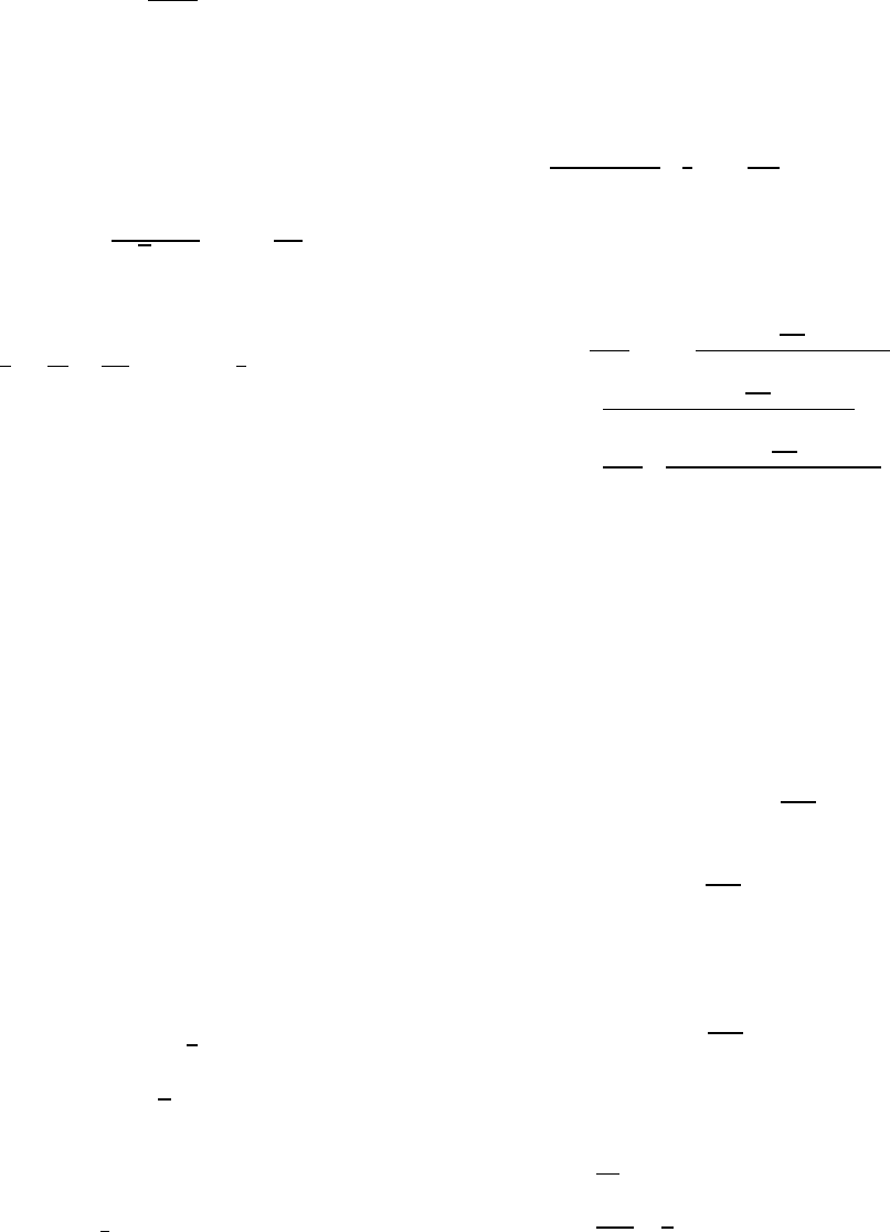
shown in Fig.1. If the power of the light-envelope
equals to the critical power, the potential will be a
constant, as can be seen by dash curve of Fig.(1).
Without the external disturbance, the light-envelope
will stay in its initial state, and keep its width change-
less. But the ideal condition without external distur-
bances can not exist in fact. If the externaldisturbance

makes the power larger than the critical power, then
the system will evolve towards the lower potential,
the beam width will become more and more smaller,
and the optical beam will collapse at last, as can be
confirmed by the dash-dot curve of Fig.1. If the ex-
ternal disturbance makes the power smaller than the
critical power, then the system will also evolve to-
wards the lower potential, the beam width will be-
come more and more larger, and the optical beam will
diffract at last, as can be confirmed by the solid curve
of Fig.1. These conclusions are consist with those
of Refs. (Berge, 1998; Moll et al., 2003; Sun et al.,
2008).
q
w
V
0
Figure 1: Qualitative plot of the potential V as a function of
q
w
for three cases, P
0
< P
c
(solid curve), P
0
= P
c
(dashed
curve), and P
0
> P
c
(dash-dot curve) when D = 2.
3.2 The Nonlocal Case
For the nonlocal case, when D ≤ 2, the condition
(37) can be satisfied automatically. That is to say the
(1+1)-dimensional and the (1+2)-dimensional nonlo-
cal solitons are always stable when the response func-
tion of the material is a Gaussian function. It is con-
sistent with the conclusion of Ref. (Bang et al., 2002).
When D > 2 the solitons can be stable only if the the
degree of nonlocality is strong enough that can satisfy
the criterion (37), which is also the same as the result
of Ref.(Bang et al., 2002).
4 TWO REMARKS
At the end, we make two remarks on the new ap-
proach in dealing with the nonlinear light-envelope
propagations presented in the paper. Firstly, the new
approach is based on the new CEH (12) and (13), and
we will show that the conventional CEH (4) and (5)
will yield contradictory and inconsistent results. Sec-
ondly, we will compare our approach with the varia-
tional approach, and discuss the differences between
them.
4.1 Contradictory Results Coming from
the Conventional CEH
Here we use the conventional CEH (4) and (5) to deal
with the light-envelope propagated in nonlinear me-
dia, following the same procedure in Sec. 3, and show
that the conventional CEH (4) and (5) will give the
contradictory and inconsistent results.
Without loss of generality, we only take the NLSE
(3) with D = 1 as an example. The NLSE is a spe-
cial case of the NNLSE when w
m
approaches to zero.
Then letting w
m
= 0 and D = 1 makes Hamiltonian
(23) reduced into
H =
√
πq
2
A
h
2
√
2−q
2
w

q
2
A
−2
√
2q
2
w
q
2
c
i
4q
w
. (40)
Because the Hamiltonian is only the function of the
generalized coordinates, the CEH (4), the right hand
side of which is the derivativeof the Hamiltonian with
respect to the generalized momentum, can yield noth-
ing unless ˙q
c
= ˙q
θ
= ˙q
A
= ˙q
w
= 0. It means the four
quantities are all the conserved quantities. This re-
sult coming from the CEH (4) is obviously wrong be-
cause such quantities as the amplitude q
A
, the width
q
w
and the phase-front curvature q
c
all generally vary
with the evolution coordinate z except for the soliton
state, and q
θ
, the phase of the complex amplitude of
the light-envelope, must be the function of z even for
the soliton state.
From the other CEH (5), four equations can be
obtained as
˙p
c
= −
∂H
∂q
c
= −
√
2πq
2
A
q
c
q
3
w
, (41)
˙p
θ
= −
∂H
∂q
θ
= 0, (42)
˙p
A
= −
∂H
∂q
A
=
√
πq
A

−
√
2+ q
2
A
q
2
w
−
√
2q
2
c
q
4
w

q
w
, (43)
˙p
w
= −
∂H
∂q
w
=
√
πq
2
A

2
√
2+ q
2
A
q
2
w
−6
√
2q
2
c
q
4
w

4q
2
w
. (44)
Substitution of the generalized momenta p
c
given
by Eq. (21) into Eq. (41) yields the same result as
Eq. (31). Then inserting Eq. (31) into the Hamiltonian
(40) gives out H =
P
0
16

˙q
2
w
+
16
q
2
w
−
8P
0
√
πq
w

. The Hamil-
tonian is the sum of the generalized kinetic energy and
the generalized potential V(q
w
) =
P
0
2

2
q
2
w
−
P
0
√
πq
w

,
which is also the same as Eq. (33) when D = 1 and
w
m
= 0. Therefore, the critical power, correspond-
ing to the extremum point of the generalized poten-
tial, P
c
=
4
√
π
q
w
is the same as Eq. (35) when D = 1
and w
m
= 0. It can also be found that Eq. (42) is the
same as Eq. (28), which means that the power of the

light-envelope is conservative. Although the first two
equations, Eqs. (41) and (42), of a set of equations
resulting from CEH (5) can give out the correct re-
sults, the other two equations, Eqs. (43) and (44), will
yield the contradictory and inconsistent results. Let
us show as follows. Inserting Eq. (20) into Eqs.(43)
and (44) yields
P
0
=
8
√
π
5q
w
, (45)
q
c
=
r
3
5
1
q
2
w
. (46)
Obviously, the two results given by Eqs. (45) and
(46) are both wrong. Under the assumption of the
light-envelope with the form of Gaussian-shape given
by Eq. (16), the power carried by the light-envelope
should be P
0
=
p
π/2q
2
A
q
w
given by Eq. (29), with
which Eq. (45) is contradictory and inconsistent.
Eq. (46) gives the fixed relation between q
c
and q
w
.
But the phase-front curvature, q
c
, should be changed
depending upon the state of the light-envelope, es-
pecially q
c
should be zero for the soliton state, with
which Eq. (46) is inconsistent.
It is no surprise to obtain such contradictory and
inconsistent results from the canonical equations of
Hamilton (4) and (5), since both the NNLSE (1) and
its complex conjugation can not be derived from the
canonical equations of Hamilton (6) and (7) as stated
in Sec. 2.
4.2 Our Approach vs the Variational
Approach: Same and Different
As mentioned above, our approach presented in this
paper is based on the canonical equations of Hamil-
ton (the Hamiltonian formulation), while the vari-
ational approach (Anderson, 1983) is based on the
Euler-Lagrange equations (the Lagrangian formula-
tion). Although the same point of the two approaches
is to first compute the Lagrangian of the system by
using a suitably chosen trial function, they are in
essence two parallel methods because the Hamilto-
nian formulation and the Lagrangian formulation are
two parallel theory frameworks in the classical me-
chanics.
The most important concept in our approach is the
“potential”. The potential given by Eq. (33) is the real
“potential” of the system that a single light-envelope
propagates in nonlocal nonlinear media modeled by
the NNLSE. It is not, of course, the potential of the
narrow-sense mechanical system, but does be the po-
tential in the frame of the Hamiltonian theory, that
is, the potential of the Hamiltonian system. In other
word, it is the potential from the Hamiltonian point of
view. Looking back to the variational approach, we
can observe that although the “potential” was also in-
troduced [see, Eqs. (28) and (29) in Ref. (Anderson,
1983)], it is just a mathematically equivalent poten-
tial in the sence that the evolution of the width of the
light-envelope can be analogous to that of a particle
in a potential well, rather than the real “potential” of
the system.
5 CONCLUSIONS
We introduce a new approach, based on the new
canonical equations of Hamilton found by us recently,
to analytically obtain the approximate solution of the
nonlocal nonlinear Schr¨odinger equation and to ana-
lytically discuss the stability of the soliton. For the
single light-envelope propagated in nonlocal nonlin-
ear media modeled by the NNLSE, the Hamiltonian
of the system can be constructed as the sum of the
generalized kinetic energy and the generalized poten-
tial. The extreme point of the generalized potential
corresponds to the soliton solution of the NNLSE.
The soliton is stable when the generalized potential
has the minimum, and unstable otherwise. In addi-
tion, we give the rigorous proof of the equivalency
between the NNLSE and the Euler-Lagrange equa-
tion on the premise of the response function with even
symmetry.
ACKNOWLEDGEMENTS
This research was supported by the National Natural
Science Foundation of China, Grant Nos. 11274125
and 11474109.
REFERENCES
Agrawal, G. (2001). Nonlinear Fiber Optics. Acadamic,
San Diego, 3rd edition.
Anderson, D. (1983). Phys. Rev. A, 27:3135.
Assanto, G. (2012a). Nematicons: Spatial Optical Solitons
in Nematic Liquid Crystals. John Wiley & Sons, New
York.
Assanto, G. (2012b). Optical Solitons: From Fibers to Pho-
tonic Crystals. John Wiley & Sons, New York.
Bang, O., Krolikowski, W., Wyller, J., and Rasmussen, J.
(2002). Phys. Rev. E, 66:046619.
Berge, L. (1998). Phys. Rep., 303:259.
Chen, L., Wang, Q., Shen, M., Zhao, H., Lin, Y., Jeng,
C., Lee, R., and Krolikowski, W. (2013). Opt. Lett.,
38:13.

Chen, X., Guo, Q., She, W., Zeng, H., and Zhang, G.
(2015). Advances in Nonlinear Optics. De Gruyter,
Berlin.
Chen, Z., Segev, M., and Christodoulides, D. (2012). Rep.
Prog. Phys., 75:086401.
Desaix, M., Anderson, D., and Lisak, M. (1991). J. Opt.
Soc. Am. A, 8:2082.
Goldstein, H., Poole, C., and Safko, J. (2001). Classical
Mechanics. Addison-Wesley.
Guo, Q., Luo, B., and Chi, S. (2006). Opt. Commun.,
259:336.
Hong, W., Guo, Q., and Li, L. (2015). Phys. Rev. A,
92:023803.
Karpman, V. and Maslov, E. (1977). Zh. Eksp. Teor. Fiz.,
73:537.
Kivshar, Y. and Agrawal, G. (2003). Optical Solitons: From
Fibers to Photonic Crystals. Elsevier, New York.
Kivshar, Y. and Malomed, B. (1989). Rev. Mod. Phys.,
61:763.
Kivshar, Y. and Pelinovsky, D. (2000). Phys. Rep., 331:117.
Krolikowski, W., Bang, O., Rasmussen, J., and Wyller, J.
(2001). Phys. Rev. E, 64:016612.
Lashkin, V., Yakimenkoa, A., and Prikhodko, O. (2007).
Phys. Lett. A, 366:422.
Liang, G., Ren, Z., and Guo, Q. (2013). Arxiv, 1311:0115.
Maimistov, A. (1993). J. Exp. Theor. Phys., 77:727.
Malomed, B., Mihalache, D., Wise, F., and Torner, L.
(2005). J. Opt. B: Quantum Semiclass. Opt., 7:R53.
Moll, K., Gaeta, A., and Fibich, G. (2003). Phys. Rev. Lett.,
90:203902.
Petroski, M., Petrovi´c, M., and Beli´c, M. (2007).
Opt.Commun., 279:196.
Picozzi, A. and Garnier, J. (2011). Phys. Rev. Lett.,
107:233901.
Seghete, V., Menyuk, C., and Marks, B. (2007). Phys. Rev.
A, 76:043803.
Silberberg, Y. (1990). Opt. Lett., 15:1282.
Snyder, A. and Mitchell, D. (1997). Science, 276:1538.
Steffensen, H., Agger, C., and Bang, O. (2012). J. Opt. Soc.
Am. B, 29:484.
Stegeman, G. and Segev, M. (1999). Science, 286:1518.
Sun, C., Barsi, C., and Fleischer, J. (2008). Opt. Express,
16:20676.
Trillo, S. and Torruellas, W. (2001). Spatial solitons.
Springer-Verlag, Berlin.
Vakhitov, N. and Kolokolov, A. (1975). Radiophys. Quan-
tum Electron., 16:783.
Wolf, E. (2002). Progress in optics. Elsevier, North-
Holland.
Zakharov, V. and Shabat, A. (1971). Zh. Eksp. Teor. Fiz.,
61:118.
Zakharov, V. and Shabat, A. (1973). Zh. Eksp. Teor. Fiz.,
64:1627.