Real-Time Prediction to Support Decision-making in Soccer

Yasuo Saito

, Masaomi Kimura

and Satoshi Ishizaki

Division of Electrical Engineering and Computer Science, Shibaura Institute of Technology, Tokyo, Japan

Department of Information Science and Engineering, Shibaura Institute of Technology, Tokyo, Japan

Health and Physical Education, Shibaura Institute of Technology, Saitama, Japan

Keywords:

Soccer, Sports Data, Game Prediction, k-NN, Clustering.

Abstract:

Data analysis in sports has been developing for many years. However, to date, a system that provides tactical

prediction in real time and promotes ideas for increasing the chance of winning has not been reported in the

literature. Especially, in soccer, components of plays and games are more complicated than in other sports.

This study proposes a method to predict the course of a game and create a strategy for the second half. First, we

summarize other studies and propose our method. Then, data are collected using the proposed system. From

past games, games to similar to a target game are extracted depending on data from their ﬁrst half. Next, similar

games are classiﬁed by features depending on data of their second half. Finally, a target game is predicted and

tactical ideas are derived. The practicability of the method is demonstrated through experiments. However,

further improvements such as increasing the number of past games and types of data are still required.

1 INTRODUCTION

Data analysis is becoming more common, including

in sports. Using data analysis results has become

familiar in sports organizations such as the Grand

Slam of the International Tennis Federation and Ma-

jor League Baseball in the USA.

Data analyses have also become popular in soc-

cer. Traditionally, in soccer, analyses were applied to

the numbers related to goals and shots. However, Shi-

genaga et al.(Shigenaga et al., 2014) used pass data,

because the number of passes is much greater than

that of goals and shots, and it provides more informa-

tion regarding the relative statuses of teams in a game.

Regarding players as nodes and passes as edges, the

motion of the ball creates a network. Shigenaga et al.

analyzed the network using graph theory and calcu-

lated centralities such as betweenness and closeness.

They determined the differences in pass networks be-

tween higher and lower ranked teams and between op-

ponents that tend to defeat a target team. From these

differences, they acquired strategies suitable for the

target team to defeat the opponent.

In fact, such analyses (Jo et al., 2014) (Yamada

et al., 2014) (Yamamoto and Yokoyama, 2011) are not

used to decide a strategy in real games. One reason is

that the motion of players and the ball is too compli-

cated to obtain data about every action that occurs in

the game. Another reason is that, since data analyses

are performed after the game, it is impossible to uti-

lize the acquired knowledge to provide advantages to

the team in the same game. Many situations such as

the conditions of players and constitutions of squads

in the team and its opponents can change every game.

This means that the most reliable data that we can use

in a game are those taken from that very game. In

fact, the number of passes and shots, percentage of

ball possessions, and covered distance of each player

are insufﬁcient to express situations in soccer games.

Therefore, it is necessary to deﬁne new data suitable

for a useful analysis.

In this study, we propose a data schema for data

necessary to measure similarity between games, and

also propose a method to predict which strategy the

target team used in past game would be expected a

good result in the target game. This can be effective

way to support decision-making regarding strategy.

Our approach is based on the assumption that games

similar in the ﬁrst half are also played similarly in the

second half. Accordingly, by applying memory-based

reasoning, we extract games similar to the target game

in the ﬁrst half at the beginning of the method. If sim-

ilar games exist, it is expected that they are ether win-

ning, drawing or losing games. If the similar games

include many winning games, their features provide

the important knowledge for decision-making in the

218

Saito, Y., Kimura, M. and Ishizaki, S..

Real-Time Prediction to Support Decision-making in Soccer.

In Proceedings of the 7th International Joint Conference on Knowledge Discovery, Knowledge Engineering and Knowledge Management (IC3K 2015) - Volume 1: KDIR, pages 218-225

ISBN: 978-989-758-158-8

target game. Even if there are only losing games in

the similar games, their feature of their games can be

useful to avoid losing in the target game. We apply

a clustering technique to classify similar games de-

pending on their features in the second half. Next, we

extract features of each groups (especially winning

game groups) by identifying data whose variance is a

minimum. Finally, we interpret the obtained features

in the games similar to the target game and predict

how the target game changes in the second half.

2 PROPOSED METHOD

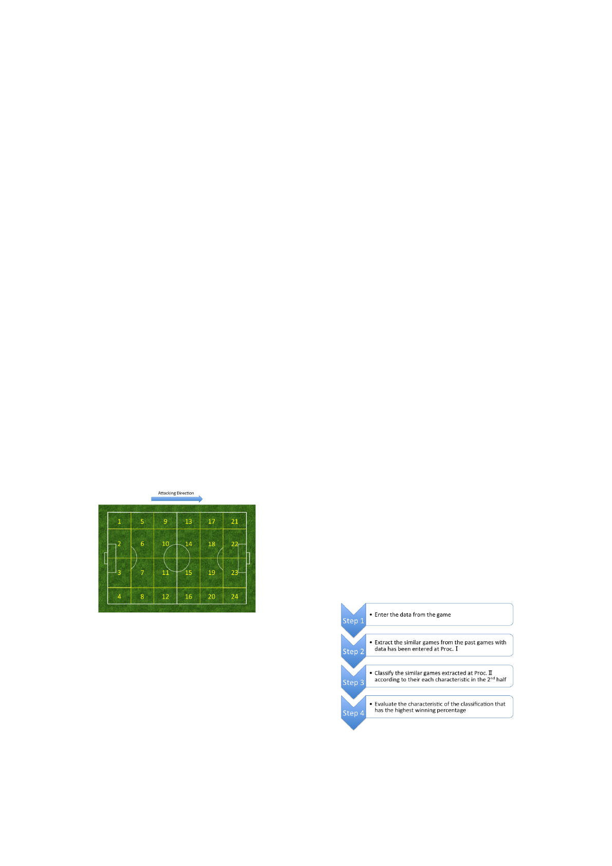
2.1 Target Data

Our target data in this approach are the zone data.

Figure 1 illustrates an image of the pitch, which is

divided into 24 parts, divided longitudinally by six

and transversally by four. The transverse division was

deﬁned to divide inside and outside the width of the

penalty box and on the left/right sides. At the World

Cup in Brazil last year, all 171 goal scorings at the

competition were made inside the width of the penalty

box. This suggests that there is a huge difference re-

garding the roles of the offense and defense depend-

ing on whether it was inside or outside the box. For

the longitudinal division, we expected to obtain infor-

mation such as efﬁciency of the attack from the ten-

dency of the longitudinal position where the ball was

frequently located.

Figure 1: Image of the pitch.

The zone data including three data types are as

follows:

• Ball Zone data (BZD)

The number of times players in a team handle with

the ball at each zone.

• Ball Interception data (BID)

The number of times players take over the ball

from their opponent players at each zone.

• Foul data (FD)

The number of times the players commit fouls at

each zone.

Moreover, we use the following statistical data

provided by Data Stadium Inc. (Data Stadium Inc.),

which handles J-League data.

• Chance percentage (the number of shots / the

number of attacks)

• Ball possessions per 15 min

• The number of shots per 15 min

• The success rate of Shot/Pass/Crosse/Take-

on/Tackle

2.2 Method

Figure 2 shows the broad outline of the technique.

The following describes each step of our method

Step 1: In this step, data are gathered by hand with

PileZD, a data input system developed by authors in

this study. Figure 3 shows its input screen. As we

showed in Section 2.1 , we use BZD, BID and FD as

original data in this method. Therefore, a user input

the type of each action that occurred in the game, such

as ball motion, ball interception and foul. Moreover,

it is also important that the position on the pitch where

each action occurred because even the type of actions

are same, they have different meanings according to

the position they happen. Therefore, it is essential

to get not only the type of action but position data.

For that reason, we developed that system to gather

data of ball motion, ball interception and foul in ev-

ery zone in the pitch as we showed in Figure 1. All

actions are able to be input their type of actions by

keyboard inputting, their zone where each actions oc-

curred by mouse clicking on the pitch in the input

screen(Figure 3). Furthermore, these data that gath-

ered with PileZD are compiled every 15 minutes and

stored into the database because it enable to reveal the

changes of the game ﬂow based on temporal game de-

velopment.

Figure 2: Outline of the process.

Real-Time Prediction to Support Decision-making in Soccer

219

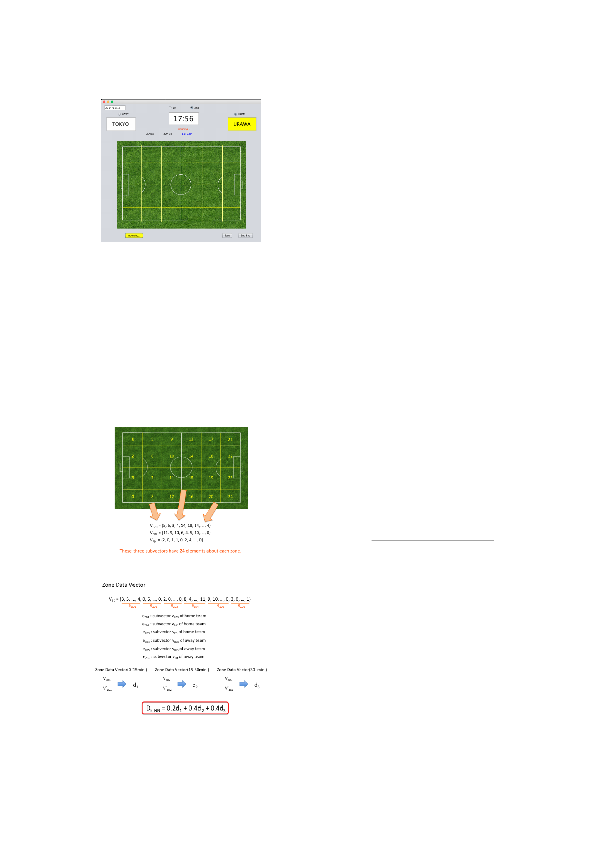
Figure 3: Input window of PileZD.

Step 2: In this method, we assume that games sim-

ilar in the ﬁrst half are also similar in the second half,

because we empirically know that opponent teams

follow a pattern in their strategies toward the target

team. Under this assumption, past games similar to

the game in progress are extracted using zone data

such as BZD, BID and FD in the ﬁrst half. Therefore,

extracted similar games will be similar to the target

game from viewpoints of ball motion, places where

the team gains/loses the ball and places the team gets

fouls.

The similarity of games is measured using the dis-

tance (Gordon S. Linoff, 1999) between vector data of

Figure 4: Creating subvectors.

Figure 5: Calculation for extraction.

game in progress and of each past game.

Figures 4 and 5 show how the distance means are

calculated. First, we create a set of subvectors of

BZD, BID, and FD for each home and away team,

as is shown in Figure 4. These subvectors have 24

elements regarding data of each zone. Then, we cre-

ate vectors by lining up each subvector in order. The

vectors v

ZD1

, v

ZD2

, and v

ZD3

in Figure 5 corresponds

to data in 0–15, 15–30, and 30 min at the end of the

ﬁrst half, respectively. All vectors have 72 elements,

which are grouped into subvectors. BZD of the home

team: e

ZD1

, BID of the home team: e

ZD2

, FD of the

home team: e

ZD2

, BZD of the away team: e

ZD6

, BID

of the away team: e

ZD6

, and FD of the away team:

ZD6

. The vectors v

ZD1

, v

ZD2

, and v

ZD3

are created

separately for the ﬁrst halves of a target game and the

past games and are used to calculate the Euclidean

distance between them. Let d

denote the distance be-

tween v

ZDi

and v

ZDi

(i = 1, 2, 3) and let the distance

of the game D

k−NN

be deﬁned as their weighted sum:

k−NN

= 0.2 d

+ 0.4 d

. We use less weight

for the ﬁrst 15 min than the others because it is not

likely that characteristic features will appear in the

ﬁrst 15 min. Applying k-NN method to the obtained

distances, the nearest k games are extracted as similar

games.

Step 3: In this step, we use a clustering algorithm

to divide similar games into multiple groups. Figure 6

shows how to calculate distances for clustering. Two

types of vectors are used: stats data vectors and zone

data vectors. Stats data vectors have 24 elements,

whose ﬁrst 12 elements, denoted as e

SD1

in Figure 6,

are the stats data for the home team, and the second

12 elements, denoted as e

SD2

are the data for the away

team. If V

and V

are vectors of any two games cho-

sen from the similar games extracted in Step 2, their

Euclidean distance d

= |V

−V

| can be obtained

SD1

− e

SD1

+ |e

SD2

− e

SD2

. (1)

Since this is a combination of stats data distances for

both teams, we adopt it as the distance between the

stats data in the second half of the game.

Here, zone data vectors are used to numerically

express the behavior of a ball in the game, whose def-

inition is the same as that in Step 2. However, in this

step, we use only one zone data vector, whose ele-

ments are the number counted in the entire of the sec-

ond half not every 15 min, as in Step 2. In our study,

we use the Euclidean distance d

between two zone

data vectors to measure their dissimilarities.

Finally, D

clustering

is the total distance between any

two games obtained in Step 2 and is calculated as the

sum of d

and d

KDIR 2015 - 7th International Conference on Knowledge Discovery and Information Retrieval

220

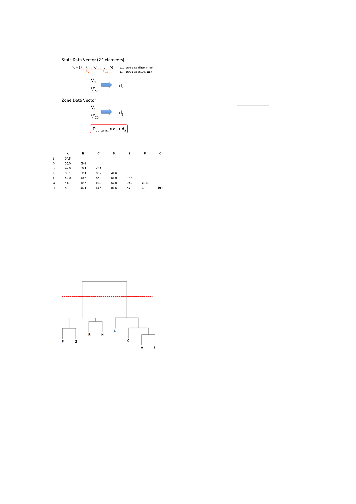
Figure 6: Calculation for clustering.

Figure 7: Example of a distance matrix.

Figure 7 is an example of a distance matrix be-

tween any two similar games. After creating this ma-

trix, to classify the games, we apply hierarchical clus-

tering (Toyoda, 2008) with Ward’s method (Toyoda,

2008) and obtain a dendrogram, as shown in Figure

8. Since the similar games can be divided into plural

groups, we chose hierarchical clustering as clustering

method to determine clusters based on the shape of

the dendrogram. In the next step, analysis of this den-

drogram reveals the features of each cluster.

Figure 8: Dendrogram.

Step 4: A threshold for dividing dendrograms into

plural clusters is determined in this step. Figure 8 is a

dendrogram based on the distance matrix in Figure7.

If it is split at the height as shown in Figure 8, all sim-

ilar games are divided into two parts: one group in-

cludes F, G, B, and H and the other group includes D,

C, A, and E. The height represents a distance thresh-

old for dividing the clusters.

After dividing similar games, we ﬁnd features of

each group according to variances of parameters such

as BZD, BID and FD in their second half. Equation

2 is the variance used in this technique, where V is

the variance of one parameter, x

is the value of the

parameter of Game i, ¯x is the average value of the pa-

rameters, and N is the number of games.

V =

∑

i=1

− ¯x)

N − 1

. (2)

Data of each parameter for all similar games are

normalized by subtracting their mean value and di-

viding by their variance (Toyoda, 2008). For each pa-

rameter, the variance is calculated, and when some

parameter has the lowest value of variance in the pa-

rameters, it is regarded as feature of the cluster. This

is because similar games in the same cluster have

close values of parameters. We take the mean value

for the parameter and interpret it by comparing with

other clusters. In this study, we employed three pa-

rameters that have the lowest variance.

3 EVALUATION

3.1 Objective and Method

The objective of this experiment is to evaluate the

proposed method by applying it to realistic data. To

simulate our method, we used 25 past J-League ofﬁ-

cial matches that Urawa Reds played in Seasons 2013

and 2014. We changed the target game and conducted

an experiment three times. Three randomly selected

games were used as target games and the other 22

games were used as past games. Before the exper-

iment, we collected BZD, BID, and FD data in the

ﬁrst and second halves and statistical data in the sec-

ond half. In these experiments, as the past games in

the ﬁrst half, we extracted eight similar games. After

the application, we calculated the winning percentage

for every cluster, discriminated which group was the

most superior, and used it to identify features that are

effective for playing the game advantageously.

On the basis of the experimental results, we dis-

cuss

• whether we can identify features that are effective

for playing the game advantageously,

• whether the actual results of the target game were

as predicted by our method.

We show the results of the experiment, in which

we used a J-League ofﬁcial game held on March 17th

2014, with Urawa Reds playing against Cerezo Os-

aka. In this game, Urawa Reds beat Cerezo Osaka by

a goal scored in the second half. We focus on whether

Urawa Reds won or lost in this section.

Real-Time Prediction to Support Decision-making in Soccer

221

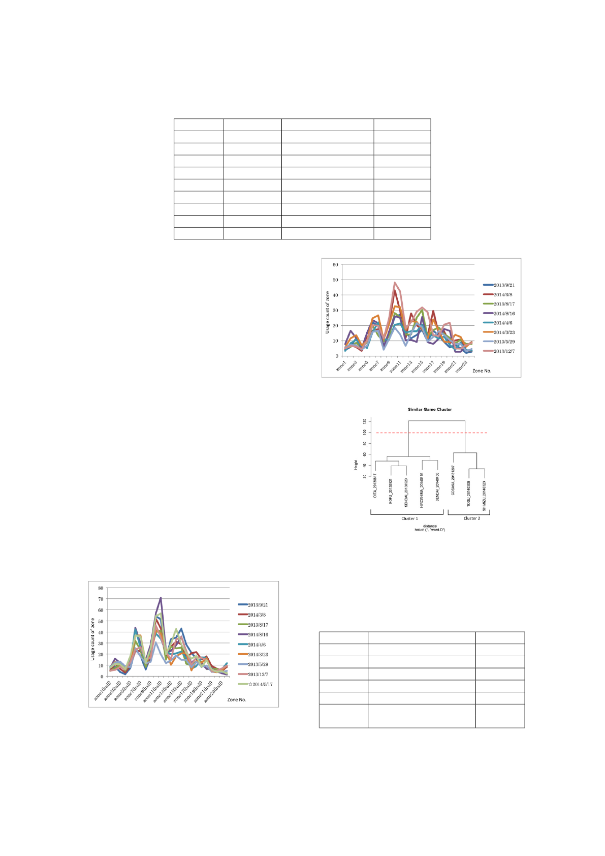
Table 1: Target game and similar games.

Distance Date Opponent teams Final score

0 (target) 2014/05/17 Cerezo Osaka 1 - 0

11.52 2013/09/21 Ventforet Kofu 1 - 1

11.91 2014/03/08 Sagan Tosu 0 - 1

13.07 2013/08/17 Oita Trinita 4 - 3

13.58 2014/08/16 Sanfrecce Hirosima 1 - 0

14.86 2014/04/06 Vegalta Sendai 4 - 0

14.88 2014/03/23 Shimizu S-Pulse 1 - 1

14.96 2013/05/29 Vegalta Sendai 1 - 1

15.03 2013/12/07 Cerezo Osaka 2 - 5

3.2 Result and Discussion

Table 1 shows the list of the target games and similar

eight games. Moreover, Figure 9 shows Urawa Reds’

BZD for every zone on the pitch in the ﬁrst half of the

target game and similar games. The horizontal axis

indicates the zone number, and the vertical axis shows

the number of times the ball was placed at the zone.

Clearly, all lines in the graph have nearly the same

shape. This indicates that the target game and similar

games have some common points in how frequently

players in Urawa Reds used zones to bring the ball.

Figure 10 shows BZDs at every zone on the pitch

in the second half of the similar games. We can see

that all the lines in the graph are similar in shape. This

indicates that the games similar in the ﬁrst half pro-

ceed similarly in the second half as well, at least in

terms of the motion of the ball. This suggests that

attacks against the same team tend to be similar re-

gardless of whether it is in the ﬁrst or second half.

We then applied cluster analysis to these similar

games and obtained the dendrogram shown in Fig-

ure 11. If we set the threshold at more than 60, we

can divide the eight similar games into two clusters,

Cluster 1 with ﬁve games and Cluster 2 with three re-

maining games. Moreover, Table 2 shows the record

difference between the two clusters. In the J-League,

Figure 9: BZD in the ﬁrst half of the target game and similar

games.

Figure 10: BZD in the second half of similar games.

Figure 11: Dendrogram of the Cluster Analysis.

a team gains three points by winning, one point by

drawing, and 0 points by losing. The index Points per

game in the table denotes the average of the points

that Urawa Reds gained in each cluster.

Table 2: Record differences between two clusters.

Cluster 1 Cluster 2

5 the number of games 3

3 - 0 - 2 Win - Draw - Lose 0 - 2 - 1

60% Winning Percentage 0%

2.2 Points per Game 0.333

8 Goal For in second half 2

2 Goal Against 3

in second half

KDIR 2015 - 7th International Conference on Knowledge Discovery and Information Retrieval

222

From Table 2, Cluster 1 can be regarded as the

cluster of the games that Urawa Reds won, because,

e.g., the winning percentage in Cluster 1 is much

greater than that in Cluster 2. This shows that we

could classify the games similar to the target game

into two clusters showing different performances. It

also suggests that we suitably selected the parameters

used in the classiﬁcation. It is important to investigate

the features of the Cluster 1 according to these ideas.

Table 3: Three lowest variances in Urawa Reds’ data in

Cluster 1.

Zone No. variance average

Zone 16 0.046 10.76

Zone 13 0.116 13.48

Zone 9 0.191 13.06

Table 3 shows three zones (or parameters in our

study) which that have the lowest variances even

though we used BZD as well as other parameters.

Consequently, we focus especially on the BZD of

games in Cluster 1.

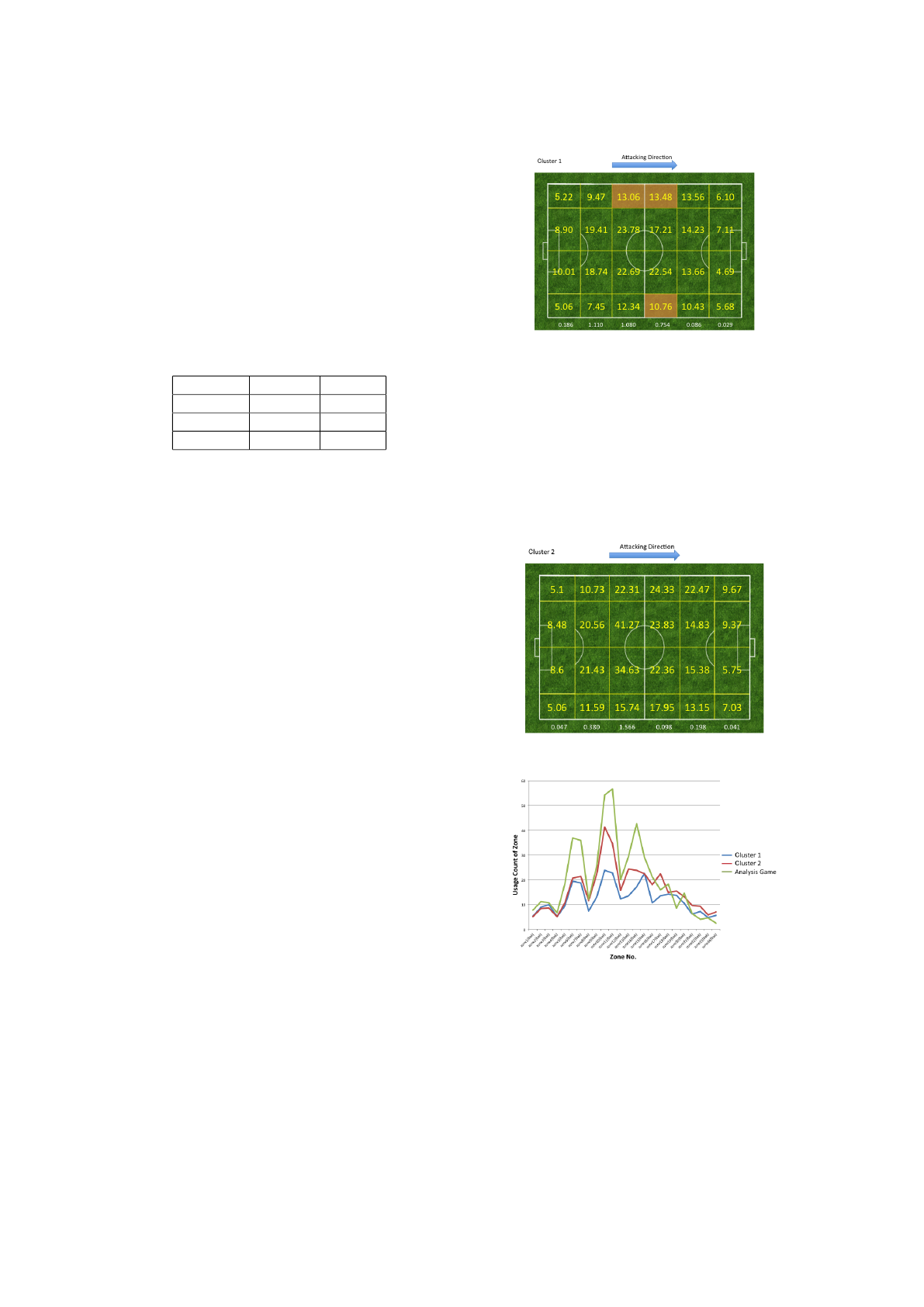
To analyze how players in Urawa Reds used each

zone for their offense, averages of BZD for each zone

are shown in their corresponding portions of the im-

age of the pitch (Figure12). Moreover, variances of

each vertical four zones are calculated and shown un-

der the pitch to ﬁnd the difference of usage in the cen-

ter and side areas. The three zones colored orange are

those with the smallest variances.

First, let us compare the data of Zones 9–16 (mid-

dle third) and Zones 17–24 (attacking third).

We can see that there are large differences in the

tendency of mean values between the middle third and

the attacking third. In the middle third, the mean val-

ues of center zones such as Zones 10, 11, 14, and 15

are clearly greater than those of outside zones, and

there are no large differences between center and out-

side areas in the attacking third. This means that in

the Cluster 1 games, Urawa Reds began their attack at

the center of the middle third, and they used the pitch

more widely toward the goal. In fact, in the game

on April 6 in 2014 between Urawa Reds and Vegalta

Sendai, all three goals that Urawa Reds scored in the

second half were the result of attacks that used both

the center and side areas in the pitch.

Similarly, by examining the mean value distribu-

tion of Cluster 2 (Figure13), we found the difference

of how Urawa Reds used the center zone and outside

of the pitch. Zones in the middle third, especially

Zones 13, 14, 15, 16, do not have clear differences

in the mean values in the center and outside. How-

ever, in the attacking third, there are large differences

in the mean value of each zone. Another point is that

Figure 12: Mean value of BZD of Cluster 1.

in the attacking third, the mean values of the left side

of the pitch (Zone 17, 21) are clearly higher than the

other area, suggesting that it is not desirable to use the

outside area unevenly in an attack.

From these results, we quantitatively conﬁrmed

that it is important to use the pitch widely and equally,

especially in front of the opponents’ goal, because

Urawa Reds played advantageously in the second half

of the target game.

Figure 13: Mean value of BZD of Cluster 2.

Figure 14: Comparison of BZD.

Finally, we compared the features of the target

game and the games in Clusters 1 and 2. Figure

14 shows the mean value of each zone. The hori-

zontal axis indicates zone numbers and the vertical

axis shows usage counts. There are three lines in the

graph: blue, red, and green lines represent Clusters 1,

Cluster 2, and the target game, respectively. We can

Real-Time Prediction to Support Decision-making in Soccer

223

see that the green line is closer to Cluster 2, which has

a lower winning percentage than Cluster 1, although

Urawa Reds ﬁnally won the target game. This might

make us think that the result of our experiment is not

as expected.

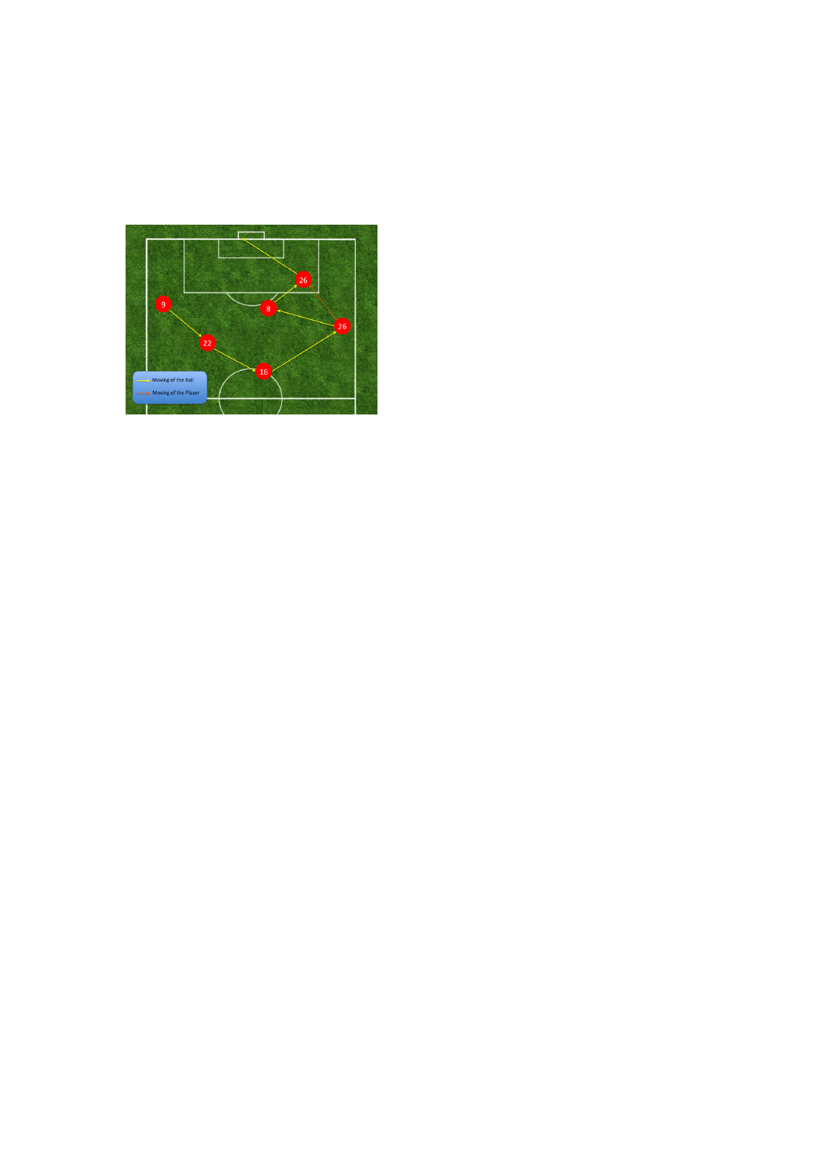
Figure 15: Goal process in the target game.

However, there were some effective attacks by

Urawa Reds in the second half of the target game.

Figure 15 shows the process of the goal that Urawa

Reds scored. It reveals that Urawa Reds used the

pitch widely, left-side, right-side, and center, a fea-

ture of attacks in Cluster 1. The reason why this oc-

cured is possibility that the distance between the sim-

ilar games and Claster 1 was wrongly calculated to be

long according to the parameters other than the scor-

ing and the used zones. Thus, in the future work, we

will need to deﬁne a distance that gives weight to the

parameters which are the features of obtained clus-

ters.

4 CONCLUSION

Recently, data analysis in sports has been developed.

Some systems have already been used to manage and

analyze data in several ﬁelds. However, so far, no

analysis method has been applied to soccer games. In

our study, we proposed a method for predicting how

games proceed in the real time.

To this end, we collected zone data (BZD, BID,

and FD) and statistical data of past games. During the

ﬁrst half of the target game, zone data were collected

and used to extract similar games from past games.

Subsequently, the extracted similar games were clas-

siﬁed by applying a clustering technique to data of

their second halves. This is because effective features

of similar games played well must also be effective in

the target game. Finally, features in the second half

in the clusters were extracted as the parameter having

the lowest variance. The information obtained was

used to discuss the strategy by which the team should

play advantageously in the second half of the target

game.

We evaluated our method by applying it to real

match data and established some points. First, we

conﬁrmed that the method extracted games similar

to the target game. Moreover, these similar games

had similar features of zone data even in their sec-

ond halves. This means that we correctly assumed

that games with similar features in their ﬁrst halves

will proceed similarly in their second halves. We

succeeded in extracting eight games from 22 past

games similar to the target game. A clustering tech-

nique revealed the difference in winning percentage

between clusters, showing that the parameters we

chose were suitable. Finally, the feature difference

between clusters that have higher and lower winning

rates were found to be closely related to strategies

that should be taken in the second half of the target

game. Though the strategy obtained was not epoch-

making, we quantitatively demonstrated an advanta-

geous strategy that is well known to people who often

watch soccer games.

In the future, we will increase the number of past

games to ensure a variety of games. In this study,

we used only zone data and a few types of statistical

data for clustering. More types of data must be used

for further analyses. Moreover, we will also need to

deﬁne a distance that gives weight to the parameters

which are the features of obtained clusters.

ACKNOWLEDGEMENTS

I wish to thank Data Stadium Inc. for providing J-

League data used in this study.

REFERENCES

Data stadium inc. https://www.datastadium.co.jp. [Online;

accessed 26-August-2015].

Gordon S. Linoff, . M. J. B. (1999). Data Mining Tech-

niques: For Marketing, Sales, and Customer Relation-

ship Management. Kaibun-do, 1st edition.

Jo, H., Yokoo, T., Ando, K., Nishijima, N., Kumagai, S.,

Naomoto, H., Suzuki, K., Yamada, Y., Nakano, T.,

and Saito, K. (2014). The attacking indexes of play-

ers and teams in j league. In Research on Sports Data

Analysis, volume 1, pages 21 – 26. The Institute of

Statistical Mathematics.

Shigenaga, K., Nakatsu, T., Naito, T., Kata, T., Saruta, S.,

Hidaka, A., Enomoto, D., Ogura, T., and Kamakura,

M. (2014). The pass analysis in soccer based on graph

KDIR 2015 - 7th International Conference on Knowledge Discovery and Information Retrieval

224

theory. In Research on Sports Data Analysis, vol-

ume 1, pages 15 – 20. The Institute of Statistical Math-

ematics.

Toyoda, H. (2008). The Guide to Data Mining with R. Toky-

oTosyo Co.,Ltd.

Yamada, M., Yagi, K., Munakata, S., Hunayama, T., and

Yamamoto, Y. (2014). The visualization of zone us-

age in soccer. In Research on Sports Data Analysis,

volume 1, pages 45 – 50. The Institute of Statistical

Mathematics.

Yamamoto, Y. and Yokoyama, K. (2011). Common and

unique network dynamics in football games. In PLos

ONE, volume 6.

Real-Time Prediction to Support Decision-making in Soccer

225