POP: A Parallel Optimized Preparation of Data for Data Mining
Christian Ernst
1
, Youssef Hmamouche
2
and Alain Casali
2
1
Ecole des Mines de St Etienne and LIMOS, CNRS UMR 6158, Gardanne, France
2
Laboratoire d’Informatique Fondamentale de Marseille, CNRS UMR 7279, Aix Marseille Universit
´
e, Marseille, France
Keywords:
Data Mining, Data Preparation, Outliers, Discretization Methods, Parallelism and Multicore Encoding.
Abstract:
In light of the fact that data preparation has a substantial impact on data mining results, we provide an original
framework for automatically preparing the data of any given database. Our research focuses, for each attribute
of the database, on two points: (i) Specifying an optimized outlier detection method, and (ii), Identifying the
most appropriate discretization method. Concerning the former, we illustrate that the detection of an outlier
depends on if data distribution is normal or not. When attempting to discern the best discretization method,
what is important is the shape followed by the density function of its distribution law. For this reason, we
propose an automatic choice for finding the optimized discretization method based on a multi-criteria (Entropy,
Variance, Stability) evaluation. Processings are performed in parallel using multicore capabilities. Conducted
experiments validate our approach, showing that it is not always the very same discretization method that is
the best.
1 INTRODUCTION AND
MOTIVATION
Parallel architectures have become a standard when
we think about modern architectures. Historically,
processors were designed to provide parallel instruc-
tions, then operating systems were built in order to ac-
cept them, in particular the task (including the thread)
manager. As a result of these advances, applications
can be distributed on several cores. Consequently,
multicore applications run faster given that they re-
quire less processor time to be executed. However,
they may need more memory since each thread re-
quires its own amount of memory.
On the other hand, many methods exist to prepare
data (Pyle, 1999), even if data preparation is few de-
veloped in the literature: The accent is more often put
on the single mining step. It is obvious that raw in-
put data must be prepared in any KDD (Knowledge
Discovery in Databases) system for the mining step.
This is for two main reasons: (i) If each value of each
column is considered as a single item, there will be a
combinatorial explosion of the search space, and thus
very large response times and/or few values returned,
and (ii) We cannot expect this task to be performed by
an expert because manual cleaning is time consuming
and subject to many errors. The data preparation step
is generally divided into:
a) Preprocessing: Which consists in reducing the
data structure by eliminating columns and rows of
low significance (Stepankova et al., 2003). Out-
liers are removed at this step. In addition, we can
perform an elimination of concentrated data by re-
moving columns having a small standard devia-
tion or containing too few distinct values;
b) Transformation: Discrete values deal with inter-
vals of values (also called bins, clusters, classes,
etc.), which are more concise for representing
knowledge, in a way that they are easier to use
and more comprehensive than continuous values.
Many discretization algorithms (see Section 4.1)
have been proposed over the years to achieve this
goal.
But data preparation often focuses on a single
parameter (discretization method, outlier detection,
null values management, etc.). Associated specific
proposals only highlight on their advantages com-
paring themselves to others. There is no global nor
automatic approach taking advantage of all of them.
However, the better data are prepared, the better
results are. Previously in (Ernst and Casali, 2011), we
proposed a simple but efficient approach for prepar-
ing input data in order to transform them into a set
of intervals to which we apply specific mining algo-
rithms to detect: Correlation Rules (Casali and Ernst,
36
Ernst, C., Hmamouche, Y. and Casali, A..
POP: A Parallel Optimized Preparation of Data for Data Mining.
In Proceedings of the 7th Inter national Joint Conference on Knowledge Discovery, Knowledge Engineering and Knowledge Management (IC3K 2015) - Volume 1: KDIR, pages 36-45
ISBN: 978-989-758-158-8
Copyright
c
2015 by SCITEPRESS – Science and Technology Publications, Lda. All rights reserved

2013), and Association Rules (Agrawal et al., 1996).
The reasons for which we have decided to reconsider
our previous work are: (i) To improve the detection
of outliers with regard to the data distribution (nor-
mal or not), (ii) To propose an automatic choice of
the best discretization method, and (iii) To parallelize
these jobs.
Globally, the objective of the presented work is
to determine automatically the values of most of the
data preparation variables, with a focus set on outlier
and discretization management. In terms of imple-
mentation, corresponding “tasks” are performed for
each attribute in parallel. And finally, we carry out
experiments.
The paper is organized as follows: Section 2
presents “current” aspects of multicore programming
we use in our work. Section 3 and Section 4 are re-
spectively dedicated to outlier detection and to dis-
cretization methods. Each Section is composed of two
parts: (i) a related work, and (ii) our approach for im-
proving it. In Section 5, we show the results of the
first experimentations. The last Section summarizes
our contribution and outlines some research perspec-
tives.
2 NEW FEATURES IN
MULTICORE ENCODING
Multicore processing is not a new concept, however
only in the mid 2000s has the technology become
mainstream with Intel and AMD. Moreover, since
then, novel software environments that are able to
take advantage simultaneously of the different exist-
ing processors have been designed (Cilk++, Open MP,
TBB, etc.). They are based on the fact that looping
functions are the key area where splitting parts of a
loop across all available hardware resources increase
application performance.
We focus hereafter on the relevant versions of the
Microsoft .NET framework for C++ proposed since
2010. These enhance support for parallel program-
ming by several utilities, among which the Task Paral-
lel Library. This component entirely hides the multi-
threading activity on the cores: The job of spawning
and terminating threads, as well as scaling the number
of threads according to the number of available cores,
is done by the library itself.
The Parallel Patterns Library (PPL) is the
corresponding available tool in the Visual C++
environment. The PPL operates on small units of
work called Tasks. Each of them is defined by a λ
calculus expression (see below). The PPL defines
three kinds of facilities for parallel processing, where
only templates for algorithms for parallel operations
are of interest for this presentation.
Among the algorithms defined as templates for
initiating parallel execution on multiple cores, we fo-
cus on the parallel invoke algorithm used in the pre-
sented work (see Sections 3.2 and 4). It executes a
set of two or more independent Tasks in parallel. An-
other novelty introduced by the PPL is the use of λ ex-
pressions, now included in the C++11 language norm:
These remove all need for scaffolding code, allowing
a “function” to be defined in-line in another statement,
as in the example provided by Listing 1. The λ ele-
ment in the square brackets is called the capture spec-
ification: It relays to the compiler that a λ function
is being created and that each local variable is being
captured by reference. The final part is the function
body.
/ / R e t u r n s t h e r e s u l t o f a d di n g a v a l u e t o i t s e l f
t e m p l a t e <typename T> T t w i c e ( c o n s t T& t ) {
r e t u r n t + t ;
}
i n t n = 5 4 ; d o u b le d = 5 . 6 ; s t r i n g s = ” He l l o ” ;
/ / C a l l t h e f u n c t i o n on ea c h v a l u e c o n c u r r e n t l y
p a r a l l e l i n v o k e (
[&n ] { n = t w i c e ( n ) ; } ,
[&d ] { d = t w i c e ( d ) ; } ,
[& s ] { s = t w i c e ( s ) ; }
) ;
Listing 1: Parallel execution of 3 simple tasks.
Listing 1 also shows the limits of parallelism. It is
widely agreed that applications that may benefit from
using more than one processor necessitate: (i) Oper-
ations that require a substantial amount of processor
time, measured in seconds rather than milliseconds,
and (ii), Operations that can be divided into signifi-
cant units of calculation which can be executed inde-
pendently of one another. So the chosen example does
not fit parallelization, but is used to illustrate the new
features introduced by multicore programming tech-
niques.
More details about parallel algorithms and the λ
calculus can be found in (Casali and Ernst, 2013).
3 DETECTING OUTLIERS
An outlier is an atypical or erroneous value corre-
sponding to a false measurement, an unwritten input,
etc. Outlier detection is an uncontrolled problem be-
cause values that are not extreme deviate too greatly
in comparison with the other data. In other words,
POP: A Parallel Optimized Preparation of Data for Data Mining
37

they are associated with a significant deviation from
the other observations (Aggarwal and Yu, 2001). In
this section, we present some outlier detection meth-
ods associated to our approach using only uni-variate
data as input.
The following notations are used to describe out-
liers: X is a numeric attribute of a database relation,
and is increasingly ordered. x is an arbitrary value, X
i
is the i
th
value, N the size of X , σ its standard devi-
ation, µ its mean, and s a central tendency parameter
(variance, inter-quartile range, . . . ). X
1
and X
N
are re-
spectively the minimum and the maximum values of
X. p is a probability, and k a parameter specified by
the user, or computed by the system.
3.1 Related Work
We discuss hereafter four of the main uni-variate
outlier detection methods.
Elimination After Standardizing the Distribution:
This is the most conventional cleaning method (Ag-
garwal and Yu, 2001). It consists in taking into ac-
count σ and µ to determine the limits beyond which
aberrant values are eliminated. For an arbitrary dis-
tribution, the inequality of Bienaym
´
e-Tchebyshev in-
dicates that the probability that the absolute deviation
between a variable and its average is greater than p is
less than or equal to
1
p
2
:
P(
x −µ
σ
≥ p) ≤
1
p
2
(1)
The idea is that we can set a threshold probability as a
function of σ and µ above which we accept values as
non-outliers. For example, with p = 4.47, the risk of
considering that x, satisfying
x−µ
σ
≥ p, is an outlier
is bounded by 0.05.
Algebraic Method: This method, presented in
(Grun-Rehomme et al., 2010), uses the relative dis-
tance of a point to the “center” of the distribution, de-
fined by: d
i
=
|
X
i
−µ
|
σ
. Outliers are detected outside of
the interval [µ −k ×Q
1
,µ + k ×Q
3
], where k is gener-
ally fixed to 1.5, 2 or 3. Q
1
and Q
3
are the first and
the third quartiles respectively.
Box Plot: This method, attributed to Tukey (Tukey,
1976), is based on the difference between quartiles
Q
1
and Q
3
. It distinguishes two categories of extreme
values determined outside the lower bound (LB) and
the upper bound (UB):
LB = Q
1
−k ×(Q
3
−Q
1
)
UB = Q
3
+ k ×(Q
3
−Q
1
)
(2)
Grubbs’ Test: Grubbs’ method, presented in
(Grubbs, 1969), is a statistical test for lower or higher
abnormal data. It uses the difference between the
average and the extreme values of the sample. The
test is based on the assumption that the data have
a normal distribution. The statistic used is: T =
max(
X
N
−µ
σ
,
µ−X
1
σ
). The tested value (X
1
or X
N
) is not
an outlier is rejected at significance level α if:
T >
N −1
√
n
s
β
n −2β
(3)
where β = t
α/(2n),n−2
is the quartile of order α/(2n)
of the Student distribution with n −2 degrees of free-
dom.
3.2 An Original Method for Outlier
Detection
Most of the existing outlier detection methods assume
that the distribution is normal. However, we found
that in reality, many samples have asymmetric and
multimodal distributions, and the use of these meth-
ods can have a significant influence at the data mining
step. In such a case, we must process each “distribu-
tion” using the appropriate method. The considered
approach consists in eliminating outliers in each col-
umn based on the normality of data, in order to mini-
mize the risk of eliminating normal values.
Many tests have been proposed in the litera-
ture to evaluate the normality of a distribution:
Kolmogorov-Smirnov (Lilliefors, 1967), Shapiro-
Wilks, Anderson-Darling, Jarque-Bera (Jarque and
Bera, 1980), etc.. If the former gives the best re-
sults whatever the distribution of the analyzed data
may be, it is nevertheless much more time consuming
to compute then the others. This is why we chosed
the Jarque-Bera test (noted JB hereafter), much more
simpler to implement as the others, as shown below:
JB =
n
6
(γ
3
2
+
γ
2
2
4
) (4)
This test follows a law of χ
2
with two degrees of
freedom, and uses the Skewness γ3 and the Kurtosis
γ
2
statistics, defined as follows:
γ
3
= E[(
x −µ
σ
)
3
] (5)
γ
2
= E[(
x −µ
σ
)
4
] −3 (6)
If the JB test is not significant (the variable is nor-
mally distributed), then the Grubbs’ test is used at a
significance level of systematically 5%, otherwise the
Box plot method is used with parameter k automati-
cally set to 3.
KDIR 2015 - 7th International Conference on Knowledge Discovery and Information Retrieval
38
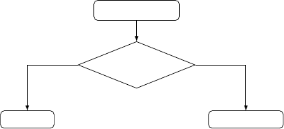
Figure 1 summarizes the process we chose to
detect and eliminate outliers.
Normality Test
Normality?
Grubbs’ Test
Box Plot
YesNo
Figure 1: The outlier detection process.
Finally, the computation of γ3 and γ2 to evalu-
ate the value of JB, so as the Grubb’s and the Box
Plot statistics calculus, are performed in parallel in the
manner shown in Listing 1 (cf. Section 2). This in or-
der to fasten the response times. Other statistics used
in the next section are simultaneously collected here.
Because the corresponding algorithm is very simple
(the computation of each statistic is considered as a
single task), we do not present it.
4 DISCRETIZATION METHODS
Discretization methods, so as outlier management
methods, apply on columns of numerical values.
However, in a previous work, we integrated also
other types of column values, such as strings, by
performing a kind of translation of such values (based
on their frequency) into numerical ones (Ernst and
Casali, 2011). This is why our approach, a priori
dedicated to numerical values, can be easily extended
to any given database.
The discretization of an attribute consists in find-
ing NbBins disjoint intervals which will further repre-
sent it in a consistent way. The final objective of dis-
cretization methods is to ensure that the mining part
of the KDD process generates efficient results. In our
approach, we use only direct discretization methods
in which NbBins must be known in advance and rep-
resents the upper limit for every column of the input
data. NbBins was a parameter fixed by the end-user
in the mentioned previous work above. As an alterna-
tive, the literature proposes several formulas (Rooks-
Carruthers, Huntsberger, Scott, etc.) for computing
such a number. Therefore we use the Huntsberger for-
mula, the best from a theoretical point of view (Cau-
vin et al., 2008), and given by: 1 + 3.3 ×log
10
(N).
We apply the formula on the non null values of each
column.
4.1 Related Work
In this section, we only discuss the final discretization
methods that have been kept for this work. This
is because other implemented methods have not
revealed themselves to be as efficient as expected
(such as Embedded Means Discretization for ex-
ample), or are otherwise not a worthy alternative to
the presented ones (Quantiles based Discretization).
The methods we use are: Equal Width Discretization
(EWD), Equal Frequency Fisher-Jenks Discretization
(EFD-Jenks), AVerage and STandard deviation
based discretization (AVST), and K-Means. These
methods, which are unsupervised and static (Mitov
et al., 2009), have been widely discussed in the
literature: See for example (Cauvin et al., 2008) for
EWD and AVST, (Jenks, 1967) for EFD-Jenks, or
(Kanungo et al., 2002), (Arthur et al., 2011) and
(Jain, 2010) for KMEANS. For these reasons, we
only summarize their main characteristics and their
field of applicability in Table 1.
Let us underline that the computed NbBins value
is in fact an upper limit, not always reached, depend-
ing on the applied discretization method. Thus, EFD-
Jenks and KMEANS generate most of the times less
than NbBins bins. This implies that other methods
which generate the NbBins value differently, for ex-
ample through iteration steps, may apply if NbBins
can be upper bounded.
Example 1. Let us consider the numeric attribute
representing the weight of several persons SX =
{59.04,60.13,60.93,61.81,62.42, 64.26,70.34, 72.89,
74.42,79.40,80.46,81.37}. SX contains 12 values,
so by applying the Huntsberger’s formula, if we aim
to discretize this set, we have to use 4 bins.
Table 2 shows the bins obtained by applying all
the discretization methods proposed in Table 1. Table
3 shows the number of values of SX belonging to each
bin associated to every discretization method.
As it is easy to understand, we cannot find two
discretization methods producing the same set of bins.
As a consequence, the distribution of the values of SX
is different depending on the method used.
4.2 Discretization Methods and
Statistical Characteristics
As seen in the last Section, when attempting to dis-
cern the best discretization method for a column, its
shape is very important. We characterize the shape
of a distribution according to four criteria: (i) Mul-
timodal, (ii) Symmetric or Antisymmetric, (iii) Uni-
form, and (iv) Normal. This is done in order to deter-
POP: A Parallel Optimized Preparation of Data for Data Mining
39
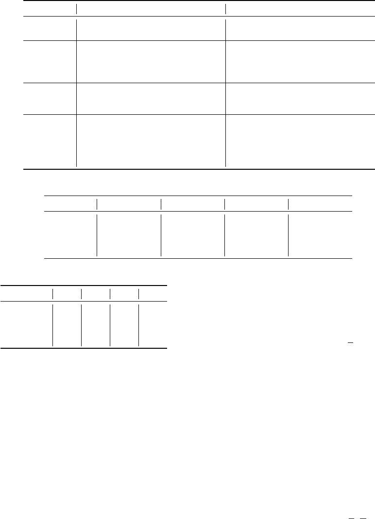
Table 1: Summary of the discretization methods used.
Method Principle Applicability
EWD This simple to implement method
creates intervals of equal width.
Not applicable for asymmetric or
multimodal distributions.
EFD-Jenks Jenks’ method provides classes with,
if possible, the same number of val-
ues while minimizing the internal
variance of intervals.
The method is effective from all sta-
tistical points of view but presents al-
gorithmic complexity in the genera-
tion of the bins.
AVST Bins are symmetrically centered on
the mean and have a width equal to
the standard deviation.
Intended only for normal distribu-
tions.
KMEANS Based on the Euclidean distance, the
method determines a partition min-
imizing the quadratic error between
the mean and the points of each in-
terval.
One disadvantage of this method is its
exponential complexity, so the com-
putation time can be long. It is appli-
cable to any form of distribution.
Table 2: Set of bins associated to sample SX.
Method Bin
1
Bin
2
Bin
3
Bin
4
EWD [59.04, 64.62[ [64.62, 70.21[ [70.21, 75.79[ [75.79, 81.37]
EFD-Jenks [59.04; 60.94] ]60.94, 64.26] ]64.26, 74.42] ]74.42, 81.37]
AVST [59.04; 60.53[ [60.53, 68.65[ [68.65, 76.78[ [76.78, 81.37]
KMEANS [59.04; 61.37[ [61.37, 67.3[ [67.3, 77.95[ [77.95, 81.37]
Table 3: Population of each bin of sample SX.
Method Bin
1
Bin
2
Bin
3
Bin
4
EWD 6 0 3 3
EFD-Jenks 3 3 3 3
AVST 2 4 4 2
KMEANS 3 3 4 2
mine what discretization method(s) may apply. Some
tests use statistics introduced in Section 3.2. More
precisely, we perform the following tests, which have
to be performed in the presented order:
Multimodal Distributions: We use the Kernel
method presented in (Silverman, 1986) to character-
ize multimodal distributions. The method is based
on estimating the density function of the sample by
building a continuous function, and then calculating
the number of peaks using its second derivative. It in-
volves building a continuous density function, which
allows us to approximate automatically the shape of
the distribution. The multimodal distributions are
those which have a number of peaks greater than 1.
Symmetric and Antisymmetric Distributions: To
characterize antisymmetric distributions in a next
step, we use the Skewness, noted γ
3
(cf. Equation (5)).
The distribution is symmetric if γ
3
= 0. Practically,
this rule is too exhaustive, so we relaxed it by impos-
ing limits around 0 to set a fairly tolerant rule which
allows us to decide whether a distribution is consid-
ered antisymmetric or not. The associated method is
based on a statistical test. The null hypothesis is that
the distribution is symmetric.
Consider the statistic: T
Skew
=
N
6
(γ
2
3
). Under the
null hypothesis, T
Skew
follows a law of χ
2
with one
degree of freedom. In this case, the distribution is
antisymmetric if α = 5% if T
Skew
> 3.8415.
Uniform Distributions: We use then the normal-
ized Kurtosis, noted γ
2
, to measure the peakedness
of the distribution or the grouping of probability den-
sities around the average, compared with the normal
distribution. When γ
2
(cf. Equation (6)) is close to
zero, the distribution has a normalized peakedness: A
statistical test is used again to automatically decide
whether the distribution has normalized peakedness
or not. The null hypothesis is that the distribution has
a normalized peakedness.
Consider the statistic: T
Kurto
=
N
6
(
γ
2
2
4
). Under the
null hypothesis, T
Kurto
follows a law of χ
2
with one
degree of freedom. The null hypothesis is rejected at
level of significance α = 0.05 if T
Kurto
> 6.6349.
Normal Distributions: We use the Jarque-Bera test
(cf. Equation (4)).
KDIR 2015 - 7th International Conference on Knowledge Discovery and Information Retrieval
40
These four successive tests allow us to character-
ize the shape of the (density function of the) distribu-
tion of each column. Combined with the main charac-
teristics of the discretization methods presented in the
last section, we get Table 4: This summarizes which
discretization method(s) can be invoked depending on
specific column statistics.
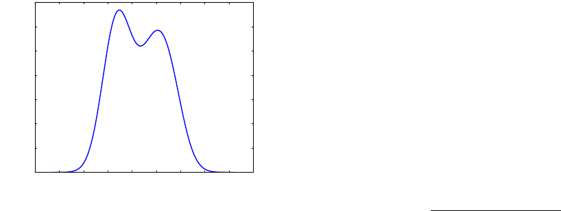
Example 2. Continuing Example 1, the Kernel Den-
sity Estimation method (Zambom and Dias, 2012) is
used to build the density function of sample SX (cf.
Figure 2).
−30 −20 −10 0 10 20 30 40 50 60
0.000
0.005
0.010
0.015
0.020
0.025
0.030
0.035
Density function
Figure 2: Density function of sample SX using Kernel Den-
sity Estimation.
As we can see, the density function has two modes,
is almost symmetric and normal. Since the den-
sity function is multimodal, we should stop at this
step. But, as shown in Table 4, only EFD-Jenks and
KMEANS produce interesting results according to our
proposal. For the need of this example, let us perform
the other tests. Since γ
3
= −0.05, the distribution is
almost symmetric. As mentioned in Section 4.2, it de-
pends on the threshold fixed if we consider that the
distribution is symmetric or not. The distribution is
not antisymmetric because T
Skew
= 0.005. The distri-
bution is not uniform since γ
2
= −1.9. As a conse-
quence, T
Kurto
= 1.805, and we have to reject the uni-
formity test. The Kolmogorov-Smirnov test results in-
dicate that the probability that the distribution follows
a normal law is 86.9% with α = 0.05. Here again,
accepting or rejecting the fact that we can consider if
the distribution is normal or not depends on the fixed
threshold.
4.3 A Multi-criteria Approach for
Finding the Best Discretization
Method
Discretization must keep the initial statistical charac-
teristics so as the homogeneity of the intervals, and
reduce the size of the final data produced. So the dis-
cretization objectives are many and contradictory. For
this reason, we chose a multi-criteria analysis to eval-
uate the available applicable methods of discretiza-
tion. We use three criteria:
1. Entropy (H): The entropy H measures the unifor-
mity of intervals. The higher the entropy, the more
the discretization is adequate from the viewpoint
of the number of elements in each interval:
H = −
NbBins
∑
i=1
p
i
log
2
(p
i
) (7)
where p
i
is the number of points of interval i
divided by the total number of points (N), and
NbBins is the number of intervals. The maximum
of H is computed by discretizing the attribute into
NbBins intervals with the same number of ele-
ments. In this case, H reduces to log
2
(NbBins).
2. Index of Variance (J): Which was introduced
in (Lindman, 2012), measures the interclass vari-
ances proportionally to the total variance. The
closer the index is to 1, the more homogeneous
the discretization is:
J = 1 −
Intra-intervals variance
Total variance
(8)
3. Stability (S): Corresponds to the maximum dis-
tance between the distribution functions before
and after discretization. Let F
1
and F
2
be the at-
tribute distribution functions respectively before
and after discretization:
S = sup
x
(
|
F
1
(x) −F
2
(x)
|
) (9)
The goal is to find solutions that present a compro-
mise between the various performance measures.
The evaluation of these methods should be done
automatically, so we are in the category of a priori
approaches where the decision-maker intervenes just
before the evaluation process step.
Aggregation methods are among the most widely
used methods in multi-criteria analysis. The princi-
ple is to reduce to a unique criterion problem. In this
category, the weighted sum method involves building
a unique criterion function by associating a weight
to each criterion (Roy and Vincke, 1981), (Cl
´
ımaco,
2012) and (Pardalos et al., 2013). This method is
limited by the choice of the weight, and requires
comparable criteria. The method of inequality con-
straints is to maximize a single criterion by adding
constraints to the values of the other criteria (Zo-
pounidis and Pardalos, 2010). Its disadvantage is
the choice of the thresholds of the added constraints.
POP: A Parallel Optimized Preparation of Data for Data Mining
41
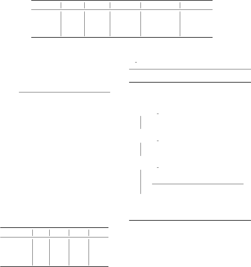
Table 4: Applicability of discretization methods = f(distribution’s shape).
Normal Uniform Symmetric Antisymmetric Multimodal
EWD * * *
EFD * * * * *
AVST *
KMEANS * * * * *
For these reasons, we chose the method that min-
imizes the Euclidean distance from the target point
(H = log
2
(NbBins), J = 1, S = 0).
Definition 1. Let D be an arbitrary discretization
method, and V
D
a measure of segmentation quality us-
ing the specified multi-criteria analysis:
V
D
=
q
(H
D
−log
2
(NbBins))
2
+ (J
D
−1)
2
+ S
2
D
(10)
The following proposition is the main result of this
article: It indicates how we chose the best method
among all the available and applicable ones.
Proposition 1. Let DM be a set of discretization
methods; the one, noted D, that minimizes V
D
(see
Equation (10)), ∀D ∈ {DM}, is the most appropriate
discretization method.
Example 3. Continuing Example 1, Table 5 shows
the evaluation results for all the discretization meth-
ods at disposal. Let us underline that for the need
of our example, all the values are computed for every
discretization method, and not only for the ones which
should have been selected after the step proposed in
Section 4.2 (cf. Table 4).
Table 5: Evaluation of discretization methods.
H J S V
DM
EWD 1.5 0.972 0.25 0.313
EFD-Jenks 2 0.985 0.167 0.028
AVST 1.92 0.741 0.167 0.101
KMEANS 1.95 0.972 0.167 0.031
The results show that EFD-Jenks and KMEANS
are the two methods that obtain the lowest values for
V
D
. The values got by the EWD and AVST methods
are the worst: This is consistent with the optimization
proposed in Table 4, since the sample distribution is
multimodal.
As a result of Table 4 and of Proposition 1, we de-
fine the POP (Parallel Optimized Preparation of data)
method, see Algorithm 1. For each attribute, after
constructing Table 4, each applicable discretization
method is invoked and evaluated in order to keep
finally the most appropriate. The content of these
two tasks (three when involving the statistics com-
putations) are executed in parallel using the paral-
lel invoke template (cf. Section 2).
Algorithm 1: POP: Parallel Optimized Preparation
of Data.
Input: X set of numeric values to discretize,
DM set of discretization methods
applicable
Output: Best set of bins for X
1 Parallel Invoke For each method D ∈ DM do
2 Compute γ
2
, γ
3
and perform Jarque-Bera
test;
3 end
4 Parallel Invoke For each method D ∈ DM do
5 Remove D from DM if it does not satisfy
the criteria given in Table 4;
6 end
7 Parallel Invoke For each method D ∈ DM do
8 Discretize X according to D;
9 V
D
=
q
(H
D
−log
2
(NbBins))
2
+ (J
D
−1)
2
+ S
2
D
;
10 end
11 D = argmin({V
D
,∀D ∈DM});
12 return set of bins obtained line 8 according to
D
5 EXPERIMENTAL ANALYSIS
In this section, we present some experimental results
by evaluating three samples. We decided to imple-
ment POP using the MineCor KDD software when
mining Correlation Rules (Ernst and Casali, 2011),
and using R Project when searching for Association
Rules. Sample
1
is a randomly generated file that con-
tains heterogeneous values. Sample
2
and Sample
3
correspond to real data representing measurements
provided by a microelectronics manufacturer (STMi-
croelectronics) after completion of the front-end pro-
cess. This is because the applicative aspect of our
work is to determine in this domain what parame-
ters have the most impact on a specific parameter, the
yield (a posteriori process control). So if the pro-
posed datasets seem a bit small, they correspond to
KDIR 2015 - 7th International Conference on Knowledge Discovery and Information Retrieval
42

Table 6: Characteristics of the databases used.
Sample Number of columns Number of rows Type
Sample
1
10 468 generated
Sample
2
1281 296 real
Sample
3
8 727 real
effective data on which we perform mining. Table 6
summarizes the characteristics of the samples.
Experiments were performed on a 4 core com-
puter (a DELL Workstation with a 2.8 GHz processor
and 12 Gb RAM working under the Windows 7 64
bits OS). First, let us underline that we shall not focus
in this section on performance issues. Of course,
we have chosen to parallelize the underdone tasks
in order to improve response times. As it is easy
to understand, each of the parallel invoke loops has
a computational time which is closed to the most
consuming calculus inside of each loop. Parallelism
allows us to compute and then to evaluate different
“possibilities” in order to chose the most efficient
one for our purpose. This, without waste of time,
when comparing to a single “possibility” processing.
Moreover, we can easily add other tasks to each
loop (statistics computations, discretization methods,
evaluation criteria), the last assertion remains true.
Some physical limits exist: No more then seven
tasks can be launched simultaneously within the
2010 C++ Microsoft .NET / PPL environment. And
each individual described task does not require more
than a few seconds to execute, even on the Sample
2
database.
Concerning outlier management, we recall that in
the previous versions of our software, we used the
single standardization method with p set by the user
(Ernst and Casali, 2011). With the new approach
presented in Section 3.2, we notice an improvement
in the detection of true positive or false negative
outliers by a factor of 2%.
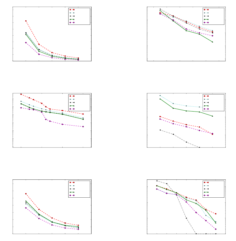
We focus hereafter on experiments performed in
order to compare the different available discretization
methods on the three samples. Figures 3(a), 4(a) and
5(a) reference various experiments when mining As-
sociation Rules. Figures 3(b), 4(b) and 5(b) corre-
spond to experiments when mining Correlation Rules.
When finding Association Rules, the minimum confi-
dence (MinCon f ) threshold has been arbitrarily set to
0.5. The different figures provide the number of Asso-
ciation or of Correlation Rules respectively while the
minimum support (MinSup) threshold varies. Each
figure is composed of five curves: One for each of the
four discretization methods presented in Table 4, and
one for our global method (POP). Each method is in-
dividually applied on each column of the considered
database.
Analyzing the Association Rules detection pro-
cess, experiments show that POP gives the best results
(few number of rules), and EWD is the worst. Using
real data, the number of rules is reduced by a factor
comprised between 5% and 20%. This reduction fac-
tor is even better using synthetic (generated) data and
a low MinSup threshold. When mining Correlation
Rules on synthetic data, the method which gives the
best results with high thresholds is KMEANS while
it is POP when the support is low. This can be ex-
plained by the fact that the generated data are sparse
and multimodal. When examining the results on real
databases, POP gives good results. However, let us
underline that the EFD-Jenks method produces unex-
pected results: Either we have few rules (Figures 3(a)
and 3(b)), or we have a lot (Figures 4(a) and 4(b)) with
a low threshold. We suppose that the high number of
used bins is at the basis of this result.
6 CONCLUSION AND FUTURE
WORK
In this paper, we presented a new approach for auto-
matic data preparation: No parameter has to be pro-
vided by the end-user. This step is generally split into
two sub-steps: (i) detecting and eliminating outliers,
and (ii) applying a discretization method in order to
transform any column into a set of bins. We show that
the detection of outliers is depending on if data distri-
bution is normal or not. As a consequence, the same
pruning method is not applied (Box plot vs. Grubb’s
test). Moreover, when trying to find the best dis-
cretization method, what is important is not the law
followed by the column, but the shape followed by
its distribution law. This is why we propose an auto-
matic choice to find the most appropriate discretiza-
tion method based on a multi-criteria approach. Ex-
perimental evaluations performed using real and syn-
thetic data validate our approach showing that we can
reduce the number of Association and of Correlation
Rules using an adequate discretization method.
For future works, we aim (i) To add other
discretization methods (Khiops, Chimerge, Fayyad-
POP: A Parallel Optimized Preparation of Data for Data Mining
43
0.005 0.010 0.015 0.020 0.025 0.030 0.035
MinSup
0
5000
10000
15000
20000
25000
30000
35000
40000
Number of Rules
EWD
AVST
EFD-Jenks
KMEANS
POP
(a) Results for APriori
0.12 0.14 0.16 0.18 0.20 0.22
MinSup
10
−1
10
0
10
1
10
2
10
3
Number of Rules
EWD
AVST
EFD-Jenks
KMEANS
POP
(b) Results for MineCor
Figure 3: Execution on Sample
1
.
0.15 0.20 0.25 0.30
MinSup
10
−1
10
0
10
1
10
2
10
3
10
4
10
5
Number of Rules
EWD
AVST
EFD-Jenks
KMEANS
POP
(a) Results for APriori
0.19 0.20 0.21 0.22 0.23 0.24 0.25
MinSup
10
1
10
2
10
3
Number of Rules
EWD
AVST
EFD-Jenks
KMEANS
POP
(b) Results for MineCor
Figure 4: Execution on Sample
2
.
0.005 0.010 0.015 0.020 0.025 0.030 0.035
MinSup
0
500
1000
1500
2000
2500
3000
3500
Number of Rules
EWD
AVST
EFD-Jenks
KMEANS
POP
(a) Results for APriori
0.04 0.06 0.08 0.10 0.12 0.14 0.16 0.18 0.20
MinSup
10
0
10
1
10
2
10
3
Number of Rules
EWD
AVST
EFD-Jenks
KMEANS
POP
(b) Results for MineCor
Figure 5: Execution on Sample
3
.
Irani, etc.) to our system, (ii) To measure the qual-
ity of the obtained rules using classification methods
(based on association rules or decision trees), (iii) To
apply our methodology with other data mining tech-
niques (decision tree, SVM, neural network) and (iv)
To perform more experiments using other databases.
REFERENCES
Aggarwal, C. and Yu, P. (2001). Outlier detection for high
dimensional data. In Mehrotra, S. and Sellis, T. K.,
editors, SIGMOD Conference, pages 37–46. ACM.
Agrawal, R., Mannila, H., Srikant, R., Toivonen, H., and
Verkamo, A. I. (1996). Fast discovery of association
rules. In Advances in Knowledge Discovery and Data
Mining, pages 307–328. AAAI/MIT Press.
Arthur, D., Manthey, B., and R
¨
oglin, H. (2011). Smoothed
analysis of the k-means method. Journal of the ACM
(JACM), 58(5):19.
Casali, A. and Ernst, C. (2013). Extracting correlated pat-
terns on multicore architectures. In Availability, Reli-
ability, and Security in Information Systems and HCI
- IFIP WG 8.4, 8.9, TC 5 International Cross-Domain
Conference, CD-ARES 2013, Regensburg, Germany,
September 2-6, 2013. Proceedings, pages 118–133.
Cauvin, C., Escobar, F., and Serradj, A. (2008). Cartogra-
phie th
´
ematique. 3. M
´
ethodes quantitatives et trans-
formations attributaires. Lavoisier.
Cl
´
ımaco, J. (2012). Multicriteria Analysis: Proceedings
of the XIth International Conference on MCDM, 1–6
August 1994, Coimbra, Portugal. Springer Science &
Business Media.
Ernst, C. and Casali, A. (2011). Data preparation in the
minecor kdd framework. In IMMM 2011, The First
KDIR 2015 - 7th International Conference on Knowledge Discovery and Information Retrieval
44
International Conference on Advances in Information
Mining and Management, pages 16–22.
Grubbs, F. E. (1969). Procedures for detecting outlying ob-
servations in samples. Technometrics, 11(1):1–21.
Grun-Rehomme, M., Vasechko, O., et al. (2010). M
´
ethodes
de d
´
etection des unit
´
es atypiques: Cas des enqu
ˆ
etes
structurelles ukrainiennes. In 42
`
emes Journ
´
ees de
Statistique.
Jain, A. K. (2010). Data clustering: 50 years beyond k-
means. Pattern Recognition Letters, 31(8):651–666.
Jarque, C. M. and Bera, A. K. (1980). Efficient tests for
normality, homoscedasticity and serial independence
of regression residuals. Economics Letters, 6(3):255–
259.
Jenks, G. (1967). The data model concept in statistical map-
ping. In International Yearbook of Cartography, vol-
ume 7, pages 186–190.
Kanungo, T., Mount, D. M., Netanyahu, N. S., Piatko,
C. D., Silverman, R., and Wu, A. Y. (2002). An effi-
cient k-means clustering algorithm: Analysis and im-
plementation. Pattern Analysis and Machine Intelli-
gence, IEEE Transactions on, 24(7):881–892.
Lilliefors, H. W. (1967). On the kolmogorov-smirnov
test for normality with mean and variance un-
known. Journal of the American Statistical Associ-
ation, 62(318):399–402.
Lindman, H. R. (2012). Analysis of variance in experimen-
tal design. Springer Science & Business Media.
Mitov, I., Ivanova, K., Markov, K., Velychko, V., Stanchev,
P., and Vanhoof, K. (2009). Comparison of discretiza-
tion methods for preprocessing data for pyramidal
growing network classification method. New Trends
in Intelligent Technologies, Sofia, pages 31–39.
Pardalos, P. M., Siskos, Y., and Zopounidis, C. (2013). Ad-
vances in multicriteria analysis, volume 5. Springer
Science & Business Media.
Pyle, D. (1999). Data Preparation for Data Mining. Mor-
gan Kaufmann.
Roy, B. and Vincke, P. (1981). Multicriteria analysis: sur-
vey and new directions. European Journal of Opera-
tional Research, 8(3):207–218.
Silverman, B. W. (1986). Density estimation for statistics
and data analysis, volume 26. CRC press.
Stepankova, O., Aubrecht, P., Kouba, Z., and Miksovsky, P.
(2003). Preprocessing for data mining and decision
support. In Publishers, K. A., editor, Data Mining
and Decision Support: Integration and Collaboration,
pages 107–117.
Tukey, J. W. (1976). Exploratory data analysis. 1977. Mas-
sachusetts: Addison-Wesley.
Zambom, A. Z. and Dias, R. (2012). A review of kernel
density estimation with applications to econometrics.
arXiv preprint arXiv:1212.2812.
Zopounidis, C. and Pardalos, P. (2010). Handbook of mul-
ticriteria analysis, volume 103. Springer Science &
Business Media.
POP: A Parallel Optimized Preparation of Data for Data Mining
45
