
Guaranteed Control of a Robotic Excavator During Digging Process
Alexander Gurko
1
, Oleg Sergiyenko
2
, Juan Ivan Nieto Hipólito
2
, Igor Kirichenko
1
,
Vera Tyrsa
3
and Juan de Dios Sanchez Lopez
4
1
Kharkov National Automobile and Highway University, Kharkov, Ukraine
2
Autonomous University of Baja California, Mexicali, Baja California, Mexico
3
Kharkiv Petro Vasylenko National Technical University of Agriculture, Kharkov, Ukraine
4
Autonomous University of Baja California, Ensenada, Baja California, Mexico
Keywords: Robotic Excavator, Guaranteed Control, Multiple Identification, R-functions.
Abstract: Automation of excavators offers a promise for increasing productivity of digging. At the same time, it’s a
highly difficult issue due to presence of various nonlinearities and uncertainties in excavator mechanical
structures and hydraulic actuators, disturbance when a bucket contacting the ground etc. This paper
concerns the problem of robust trajectory tracking control of an excavator arm. To solve this problem, the
computed torque control with the guaranteed cost control is considered. The mathematical tool of R-
functions as an alternative to the linear matrix inequality approach to constructing information sets of an
excavator arm state is used. Simulation results and functional ability analysis for the proposed control
system are given.
1 INTRODUCTION
Hydraulic excavators are used at a wide variety of
sites from civil construction to disaster elimination,
therefore efficiency and productivity increase of
these machines is a highly important problem. One of
the ways to solve the problem is to design a robotic
excavator. In addition to the increase of productivity,
the automation of excavators reduces loads on an
operator, improves his safety and makes it possible to
work in places that are inaccessible for humans.
However, robotic excavators are created
extremely slowly due to high dynamic loads during
the bucket and soil interaction, which is difficult to
predict, and other uncertainties such as backlashes
between machine parts, variability of a fluid
viscosity in hydraulic actuators, oil leaks, etc.
There are a lot of papers focused on the robotic
excavator design and creation of digging process
control system. For example, some works (Koivo et
al, 1996; Gao et al., 2009; Gu et al., 2012) describe
PD and PID controllers application to control a
robotic excavator arm movement. Besides, in one of
the papers (Gu et al., 2012) a proportional-integral-
plus (PIP) controller and a nonlinear PIP controller
based on a state-depended parameter model structure
were proposed.
In one of the works (Yokota et al., 1996) a
disturbance observer in addition to PI-controller to
control a mini excavator arm was proposed. Along
with the computed torque control, the adaptive and
robust controls of the excavator arm were designed in
(Yu et al., 2010).
In (Bo et al.) a fuzzy plus PI controller with fuzzy
rules based on the soft-switch method was
developed. In (Zhang et al., 2010) an adaptive fuzzy
sliding mode control to realize the trajectory tracking
control of an automatic excavator was designed. Two
controllers based on fuzzy logic, including the fuzzy
PID controller and fuzzy self tuning with neural
network, were developed in (Le Hanh et al., 2009) to
control the electro hydraulic mini excavator. In
(Choi, 2012) the Time-Varying Sliding Mode
Controller with fuzzy algorithm was applied to the
tracking control system of the hydraulic excavator.
Time-delay controllers were proposed for motion
control of a hydraulic excavator arm in (Chang and
Lee, 2002; Vidolov, 2012).
All these works have made a valuable
contribution to solve the problem of robotic
excavator creating, but a commercial fully robotic
excavator will probably appear not soon due to the
mentioned above factors.
In this paper we propose the guaranteed cost
control for the trajectory tracking control of the
52
Gurko A., Sergiyenko O., Hipólito J., Kirichenko I., Tyrsa V. and Lopez J..
Guaranteed Control of a Robotic Excavator During Digging Process.
DOI: 10.5220/0005536000520059
In Proceedings of the 12th International Conference on Informatics in Control, Automation and Robotics (ICINCO-2015), pages 52-59
ISBN: 978-989-758-123-6
Copyright
c
2015 SCITEPRESS (Science and Technology Publications, Lda.)
excavator arm during digging operation. The control
guarantees the robustness against uncertainties of
modelling and unexpected disturbances due to, for
instance, the bucket and soil interaction.
2 EXCAVATOR MODELLING
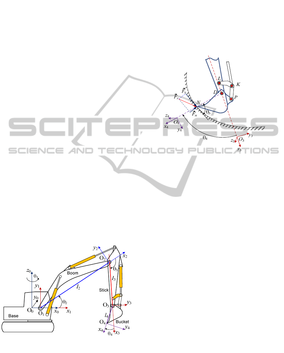
2.1 Modelling of an Excavator Arm
The dynamic model of an excavator arm can be
obtained using the Lagrange equation and can be
expressed concisely in matrix form as the well-
known equations for a rigid-link manipulator (Spong
et al, 2006):
() (,) () ()
L
DC GB
,
(1)
where
,,
are the 41 vectors of the measured
joint position, velocity and acceleration angles as
shown in Figure 1;
()D
is the 44 symmetric,
positive-definite inertia matrix;
(,)C
is the 44
Coriolis and centripetal matrix;
()G
is the 41
vector of gravity terms;
()B
is the 41 vector of
frictions;
is the 41 vector specifying the torques
acting on the joint shafts; and
L
is the 41 vector
representing the interactive torques between the
links and environment during the digging operation.
For the convenience, dynamic equation (1) can
be rewritten as follows:
() (,)
L
DN
.
(2)
where
(,) (,) () ()NCGB
.
Figure 1: Coordinate frames of an excavator.
Note that since during the digging operation the
joint variable
1
is not changed, it is therefore
assumed that
11
0
.
2.2 Digging Resistance Force
Digging by an excavator is performed due to the
bucket movement in two directions. The main
movement, named lifting, cuts a slice of soil. The
second movement (penetration) is perpendicular to
the main movement and regulates the thickness of
the cut slice of the soil.
Figure 2: Bucket and soil intersection.
During digging of soil by an excavator there acts a
resistance force
r
F
at the cutting edge of the bucket
teeth (Figure 2).
r
F
is a resultant reaction force of the
tangential
t
F
and the normal
n
F
forces. According
to M.G. Dombrovskij (Alekseeva et al. 1985), the
tangential force can simplistically be determined as
t с
F
kbh
,
(3)
where
с
k
is the specific cutting force in N/m
2
that
takes into account soil resistance to cutting as well
as all other forces (frictional resistance of the bucket
with the ground, resistance to the movement of the
prism of soil etc.); h and b are the thickness and
width of the cut slice of soil.
The normal component
n
F
is calculated as:
nt
F
F
,
(4)
where is a dimensionless factor depending on the
digging angle, digging conditions and the cutting
edge where = 0.1–0.45. Higher values of
corresponds to more dulling of the bucket teeth edge.
Thus, the torques of resistance forces for each
link of an excavator arm can be calculated as:
2
3
4
111
011
001
L
LL
L
,
(5)
GuaranteedControlofaRoboticExcavatorDuringDiggingProcess
53

where
44
sin cos
L
tbn b
lF F
;
33 4 4
sin( ) cos( )
Lt bn b
lF F
;
22 34 34
sin( ) cos( )
L
tbn b
lF F
;
b
is the angle between the axes
4
x
and the
direction of the force
t
F
(Figure 2);
34 3 4
(Figure 1);
j
l
,
2,4j
are the lengths of the
excavator arm links.
It is obvious that using more accurate models of
a bucket and soil interaction, for example given in
(Luengo, 1998), still possible improve the
performance of proposed control system.
2.3 Controller Model
In classical case of manipulator control, the
computed-torque control (CTC) and computed-
torque-like controls are widely used.
The equation for the CTC is given by Spong
(Spong et al., 2006)
() (,)
L
uD aN
,
(6)
where u is the control vector;
d
vp
aKeKe
;
p
K
and
v
K
are symmetric positive-definite matrices;
d
e
is the position error vector;
d
e
is the
velocity error vector; and superscript “d ” means
“desired”.
As far as the values of the parameters in (2) are
not known exactly due to the uncertainties in the
system, we have to rewrite the control (6) as
ˆˆ
() (,)
L
uD aN
,
(7)
where the notation
()
represents the estimates of
the terms in the dynamic model.
Having substituted (7) in (2), we can obtain
a
, where
is the uncertainty. Hence,
d
ea
. We can set the outer loop control as
aa
, where
a
is to be chosen to guarantee
robustness to the uncertainty effects
. By taking
[]
TTT
x
ee
as the system state, the following
first-order differential matrix equation is obtained:
()
x
Ax B a
,
(8)
where
A
and B are the block matrices of the
dimensions (66) and (63) respectively:
0
pv
E
A
KK
;
0
B
E
.
Thus, the issue of the control of an excavator
arm movement is reduced to finding an additional
control input
a
to overcome the influence of the
uncertainty
in the nonlinear time-varying system
(7) and to guarantee ultimate boundedness of the
state trajectory x in (8).
3 CONTROLLER DESIGN
3.1 Kinematic Control
Previously to development of control system as
subject to improve an excavator dynamics, it is
necessary to solve the problem of its kinematic
control. In (Sergiyenko et al., 2013) it was
considered an optimal solution of inverse kinematics
task for robotic excavator that provides bucket teeth
movement along the desired path. As optimality
criterion the minimizing of quadratic function (9) of
joint angles associated with the respective weights
was accepted:
4
2
0
0
2
min
I
jjj
j
J
θ
,
(9)
where
0
j
and
I
j
are the initial and the final values
of the angles
j
,
2,4j
, respectively (Figure 1);
j
are the weighting factors, that prioritize the
angles changing
j
;
is the given subset.
To solve the problem (9) it is necessary to solve
the matrix equation (10):
ii i
H
F
,
(10)
where
234
[]
iiiT
i
;
i
j
are increments of
the joint angles of an excavator arm at each step i in
time domain;
[]
iiT
ibb
F
xz
;
i
b
x
and
i
b
z
are
increments of a bucket teeth coordinates in a
Cartesian frame at each i-th step in time domain;
44
111
44
23
44
111
44
23
sin sin sin
cos cos cos
iii
jj jj
jj
i
iii
jj jj
jj
lll
H
lll
;
2
j
jk
k
,
2,4j
.
Using the Tikhonov's regularization method we
can write the original equation (10) in the next form
ICINCO2015-12thInternationalConferenceonInformaticsinControl,AutomationandRobotics
54

TT
ii i ii
H
HHF
,
(11)
where is arbitrary small positive parameter that
provides stability of the matrix
1
()
T
ii
HH
computation; is the square 3×3 matrix.
In classical problems the matrix has equal
diagonal elements. Taking into account the specifics
of the vector
i
, we will use the diagonal matrix
which non-zero elements are defined as:
1, 1jj
j
,
2,4j
.
(12)
If the values of
j
are known, solution of (12) is
trivial.
The weighting coefficients
j
we propose to
define in next way. The value of
2
is selected
wittingly large to minimize the boom motion.
Values
3
and
4
depend on the method of digging:
- when digging with the bucket
3
>>
4
;
- when digging with the stick
4
>>
3
;
- when excavator digs simultaneously with the
stick and with the bucket, the
3
and
4
ratio is
chosen to equate the maximum angular acceleration
of
3
and
4
. Accelerations
j
are calculated by the
well-known formula:
11
2
2
iii
jjj
i
j
t
.
(13)
3.2 Robust Control
For an additional control
a
determining, we
propose the optimal guaranteed cost control
approach. According to this approach, it is assumed
that uncertainties in the system are known with
accuracy to a certain guaranteed bounded set.
During the control system operation the new sets
representing the estimates of the system state are
built. The advantage of this approach is in providing
an upper bound on a given performance index and
thus, the system performance degradation incurred
by the uncertainties is guaranteed to be less than this
bound (Gurko, et al., 2012).
Let's derive the digital version of the equation
(8) for the digital control system implementation:
1
{ } ( 0,1,..., 1)
kdkdkk
xAxB ak n
,
(14)
where
d
A
and
d
B are the digital versions of the
matrices
A
and B in (8); the uncertainty
k
is
bounded by the known set
k
; k – moments of
quantization.
Control is formed on the basis of joint angles
measurements are represented in the form of the
vector
k
y
:
( ), ( 1,2,..., 1)
kdkk
yCxv k n
.
(15)
where
d
C
is the output matrix;
k
v
is the vector of
measurement noises bounded by the known set
v
k
.
As the aim of the control we assume the
minimizing of the following cost function:
1
(, ) ( ) (, )
kk k kk kk k
J
xa Vx xa
,
(16)
where
k
V
is Lyapunov function that allows
estimating the quality of the further excavator arm
motion in the absence of perturbations;
k
is the
given function, which defines the control costs and
assigns limitations on their value.
For the well-posed task (16) formulation,
information about the uncertainty
k
has to be
redefined. As far as the
k
can take on any value
inside the set
k
, we have to consider the values
maximizing the cost function (16).
Moreover, the fact that
k
and
k
v belong to the
proper sets
k
and
v
k
enables to suppose that as a
result of measurement (15) of the excavator arm
joint angles , information about the current state is
obtained in the form of the set
r
kk
x
. For the
additional control
a
determining the point
estimation of
r
kk
x
is required. For this purpose
we will consider the point maximizing the cost
function (16). So, the objective of the additional
control
k
a
is to solve the following task:
min max max max ( , )
u
vr
k
kk
k
k
kk
k
kk k
a
vx
J
xa
.
(17)
It’s obvious that the task (17) solution guarantees
the proper excavator control system performance
that depends on
k
J
at any allowed
k
and
k
v .
The description of the sets of the possible states
of the excavator arm we will carry out according to
following algorithm (Gurko at al., 2012).
1. Let at an arbitrary moment of quantization k
there is an estimate of the excavator arm state as
r
kk
x
. The transformation (18) should be realised
to find the set of states
,1
f
kk
,1
f
r
dk
kk
A
,
(18)
where
,1
f
kk
is a prediction of possible system
states
1,1
ff
kkk
x
at the
[1]k
th moment to which
GuaranteedControlofaRoboticExcavatorDuringDiggingProcess
55
it must transit moving freely from the state
r
kk
x
.
2. A new set
,1
w
kk
of possible system states is
developed by transformation (blurring) of the set of
states
,1
f
kk
:
,1
,1
f
w
kk d
kk k
B
,
(19)
where
k
is the aggregate of boundary elements
of the set
k
.
Thus, the set
,1
w
kk
is a prediction of the
excavator arm state at the [k + 1]th moment with
allowance for the influence exerted by uncertainties
k
on values of parameters of the vector
1
f
k
x
.
3. A value
1,1
uw
kkk
x
of the system state is
found. The
1
u
k
x
is used for an additional control
k
a
determined to solve the task (16).
4. The moving of the set
,1
w
kk
by the
additional control
k
a
is provided and a new set
1
u
k
is constructed. The set
1
u
k
is an estimation
of the system state to which it must transit at the
[k + 1]th moment under
k
a
and
k
action.
5. The new measurement of joint angles
k
is
carried out to find a posteriori estimate
11
r
kk
x
of the system state at the [k + 1]th moment:
11 1
ru v
kk k
.
(20)
Further, the mentioned procedure is repeated
iteratively.
4 DETERMINING A SET OF
POSSIBLE STATES
Until recently linear matrix inequalities have been
used to construct sets of control system possible
states. In (Gurko and Kolodyazhny, 2013) we
proposed to use R-functions for this purpose. This
significantly simplifies the estimation of a control
system state.
The R-function
()
k
x
of the set
k
has the
following properties:
()0,when ,
()0,when ,
()0,when ,
kkk
kkk
kkkk
xx
xx
xx
where
k
is the aggregate of boundary elements
of the set
k
.
Let’s denote R-functions of the sets
r
k
,
,1
f
kk
,
k
,
v
k
,
u
k
and
,1
w
kk
as
()
r
k
x
,
()
f
k
x
,
()
k
x
,
()
v
k
x
,
()
u
k
x
and
()
w
k
x
. For
instance, the set
r
k
is constructed using the
following R-function:
() () ()
ru v
kkk
R
x
xx
,
(21)
where
R
is the R- operation of conjunction:
22
() ()
uvuv u v
R
.
(22)
5 SIMULATIONS
A simulation study of the excavator arm motion with
the numerical values given in Table 1 (Koivo et al,
1996) was performed in MATLAB.
Table 1: Excavator parameters.
Link Mass, kg
Inertia, kgm
2
Length, m
Boom 1566 14250.6 5.16
Stick 735 727.7 2.59
Bucket 432 224.6 1.33
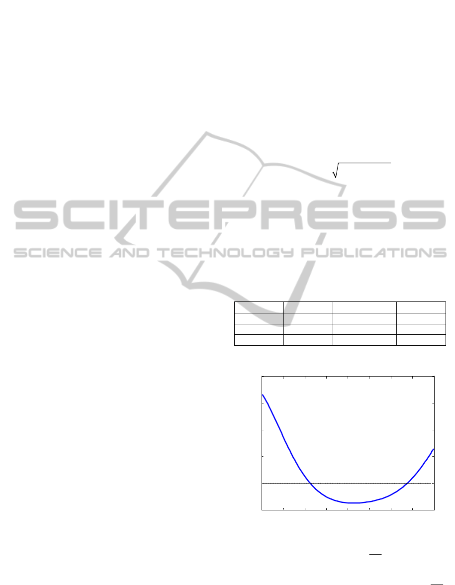
A bucket desired trajectory is presented in Figure 3.
Figure 3: Bucket desired trajectory.
The desired joint angles
j
,
2,4j
was calculated
by the equation (11) and are shown in Figure 4.
At simulating only the joint angles
j
,
2,4j
have been measured. It was assumed that the
measurement noise is in the foregoing range
3.5 4 4.5 5 5.5 6 6.5 7 7.5
-0.5
0
0.5
1
1.5
2
Ground level
x, m
z, m
ICINCO2015-12thInternationalConferenceonInformaticsinControl,AutomationandRobotics
56
0.5
i
v
deg and is subject to the uniform
distribution law. The resistance forces experienced
when the bucket penetrates into the soil are
calculated by (3)-(4).
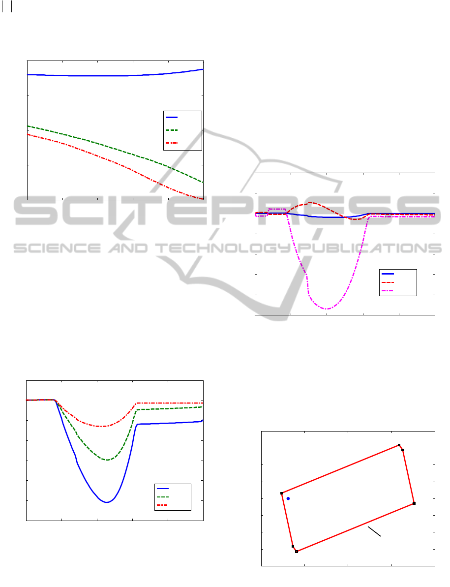
Figure 4: Desired angles.
Loam as the type of soil has been considered; the
loam density varied arbitrarily in the range
1600
s
1900 kg/m
3
. The exact value of the force
k
c
in (3) was considered to be unknown except for
the fact that it belongs to the set
117600 k
c
245000 N/m
2
. The value of the factor
in (4) was assumed to be 0.25. Changing of the
bucket mass has been also taken into account. The
true load torques
L
acted at the links are shown in
Figure 5.
Figure 5: Load torques
L
acted at the links.
As the aim of the control the task (16)-(17)
solution has been assumed, where
11
T
kk k
VxPx
;
T
kkk
aRa
;
{0.7,0.5,0.2}Rdiag
and
3.2 0 0 1.12 0 0
03.20 01.120
003.2001.12
1.12 0 0 1.86 0 0
01.120 01.860
0 0 1.12 0 0 1.86
P
.
Sampling time was T
s
= 0.1 s. For the sets of the
system possible states R-functions have been used.
The simulation results are presented in
Figures 6-8. As depicted in Figure 6, the joint angles
tracking errors are less than 0.1, 0.2, and 1 degrees
for the boom, stick and bucket, respectively.
Figure 6: Joint angles tracking errors versus time.
In Figure 7 the predicted sets of possible states
r
vs. the true system states x
t
at t = 4 s are shown.
It corresponds to the maximum value of the bucket
tracking error. For the sets
r
determine the
expressions (18) - (20) have been used.
Figure 7: Predicted sets
r
and the true system states X
t
: a
– for the boom; b – for the stick; c – for the bucket.
0 2 4 6 8 10
-150
-100
-50
0
50
t, s
Desired angles
j
, deg
Boom
Stick
Bucket
0 2 4 6 8 10
-3
-2.5
-2
-1.5
-1
-0.5
0
0.5
x 10
5
t, s
L
, N/m
2
Boom
Stick
Bucket
0 2 4 6 8 10
-1
-0.8
-0.6
-0.4
-0.2
0
0.2
0.4
t, m
Tracking error, deg
Boom
Stick
Bucket
-2 -1 0 1 2
x 10
-3
-0.02
-0.015
-0.01
-0.005
0
0.005
0.01
0.015
0.02
X
t
x
2
, rad
d
x
2
, ra
d/
sec
t, s
a
r
GuaranteedControlofaRoboticExcavatorDuringDiggingProcess
57
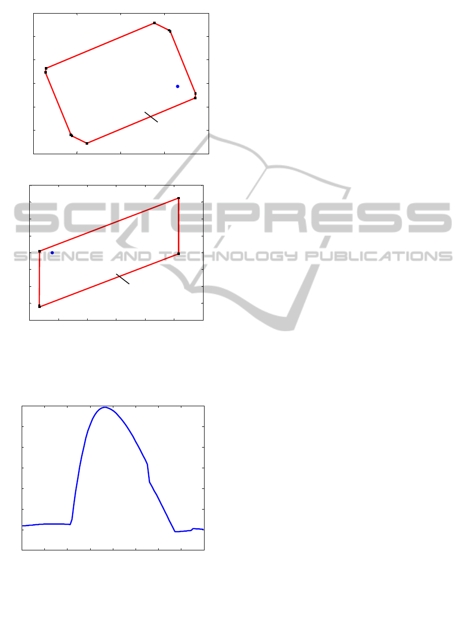
Figure 7: Predicted sets
r
and the true system states X
t
: a
– for the boom; b – for the stick; c – for the bucket (cont.).
The digging error is less than 1.2 cm or 3.5%
(Figure 8).
Figure 8: Digging error.
The simulation results illustrate that the proposed
controller provides high quality of digging under
uncertainties.
6 CONCLUSIONS
The work presented in this article investigates a new
controller to do digging trajectory tracking for a
robotic excavator. The controller requires two
circuits: the first circuit calculates the main control
using the CTC, and the aim of the second one is to
provide an additional control to compensate effect of
uncertain factors on the basis of differential games
with quadratic cost.
The mathematical tool of R-functions as the
alternative of the linear matrix inequality approach
to constructing information sets of the excavator arm
state is used.
The practical value of the proposed controller is
in providing an upper bound on a given performance
index at any uncertainties from the given bounded
set, as well as in requiring a relatively low
computational capability compared to other
reviewed methods.
Since the uncertainties do not always tend to
maximize the cost function, the implementation of
an additional circuit of adaptation which adjusts the
bounds of sets of uncertain parameters is desirable.
Our future work will investigate this aspect.
REFERENCES
Alekseeva, T. V., Artem’ev K. A., et al., 1985. Machines
for Earthmoving Work. Theory and Calculations,
Amerind Publishing. New Delhi.
Bo, L., et al., 2011. High performance control of hydraulic
excavator based on fuzzy-PI soft-switch controller. In
IEEE International Conference on Computer Science
and Automation Engineering (CSAE), vol. 2,
pp. 676-679.
Chang, P. H., Lee S. J., 2002. A straight-line motion
tracking control of hydraulic excavator system.
Mechatronics, vol. 12, No. 1, pp. 119-138.
Choi, J., 2012. Tracking control of hydraulic excavator
using time varying sliding mode controller with fuzzy
system. Advanced Science Letters, vol. 15, No 1,
pp. 78-82.
Gao, Y., et al., 2009. Motion planning based coordinated
control for hydraulic excavators. Chinese Journal of
Mechanical Engineering, vol. 22, No. 1, pp. 97-101.
Gu, J., Taylor, J., Seward, D., 2004. Proportional-Integral-
Plus Control of an Intelligent Excavator. Computer-
Aided Civil and Infrastructure Engineering, vol. 19,
No 1, pp. 16-27.
Gurko, A. G., et al., 2012. Robust Control of Excavation
Mobile Robot with Dynamic Triangulation Vision. In
ICINCO 2012, 9th International Conference on
Informatics in Control, Automation and Robotics,
vol. 2, pp. 481-484.
-4 -2 0 2 4
x 10
-3
-0.06
-0.04
-0.02
0
0.02
0.04
0.06
X
t
x
3
, rad
dx
3
, rad/sec
-0.018 -0.016 -0.014 -0.012 -0.01 -0.008 -0.006
-8
-6
-4
-2
0
2
4
6
8
x 10
-3
X
t
x
4
, rad
dx
4
, rad/sec
3.5 4 4.5 5 5.5 6 6.5 7 7.5
-0.2
0
0.2
0.4
0.6
0.8
1
1.2
x, m
Digging error, cm
b
c
r
r
ICINCO2015-12thInternationalConferenceonInformaticsinControl,AutomationandRobotics
58

Gurko, A. G., Kolodyazhny, V. M., 2013. Estimating the
State Vector of a Dynamic System under Uncertainty.
Cybernetics and Systems Analysis, vol. 49, No 6,
pp. 821-828.
Koivo, A. J., et al., 1996. Modeling and Control of
Excavator Dynamics During Digging. Journal of
Aerospace Engineering, vol. 9, No. 1, pp. 10-18.
Le Hanh, D., et al., 2009. Trajectory control of electro-
hydraulic excavator using fuzzy self tuning algorithm
with neural network. Journal of Mechanical Science
and Technology, vol. 23, No 1, pp. 149-160.
Luengo O., et al., 1998. Modeling and identification of
soil-tool interaction in automated excavation. In
IEEE/RSJ International Conference on Intelligent
Robots and Systems, vol. 3, pp. 1900-1906.
Nguyen, Q.H., et al., 1999. Feedback linearization control
for electro-hydraulic systems of a robotic excavator. In
Proceedings of the Australian Conference on Robotics
and Automation, Brisbane, Australia, pp. 190-195.
Sergiyenko, O. Yu., et al., 2013. Optimal Kinematic
Control of a Robotic Excavator with Laser TVS
feedback. In IECON 2013, 39th Annual Conference of
the IEEE Industrial Electronics Society, pp. 4239-
4244.
Spong, M. W., Hutchinson, S., Vidyasagar, M., 2006.
Robot modeling and control, Wiley. New York, 1
st
edition.
Vidolov, B., 2012. A Discrete-Time Design of Time Delay
Control Focus on Control Experimentations of
Coordinated Motion Control of Hydraulic Excavator.
In SYROCO’12, 10th International IFAC Symposium
on Robot Control, Dubrovnik, Croatia, pp. 6.
Yokota, S., et al., 1996. Trajectory Control of the boom
and arm system of hydraulic excavators. Transactions
of the Japan Society of Mechanical Engineers, part C,
vol. 62, No. 593, pp. 161-167.
Yu, H., et al., M. S, 2010. Review of modelling and remote
control for excavators. International Journal of
Advanced Mechatronic Systems, vol. 2, No 1, pp. 68-80.
Zhang, J., et al., 2010. 4-DOF Adaptive Fuzzy Sliding
Mode Control of Excavator. Jixie Gongcheng Xuebao
(Chinese Journal of Mechanical Engineering), vol.46,
No 21, pp. 87-92.
GuaranteedControlofaRoboticExcavatorDuringDiggingProcess
59
