Gaussian Mixture Measurements for Very Long Range Tracking

Qian Zhang, Taek Lyul Song

Department of Electronic Systems Engineering, Hanyang University, Hanyang, Republic of Korea

eywords:

Nonlinear Estimation, Very Long Range Tracking, Gaussian Mixtures, GMM-ITS.

Abstract:

Target tracking with very long range is studied in this paper. Such tracking problem has severe measurement

nonlinearity that will cause consistency problems and large tracking errors. Gaussian mixture measurements

are obtained by dividing the measurement likelihood into several Gaussian components. The Gaussian Mixture

Measurement-Integrated Track Splitting (GMM-ITS) is applied to very long range tracking scenarios. The

simulation results show that the GMM-ITS can produce consistency in the ﬁltering results crucial to the ﬁlter

performance. Furthermore, it is also able to estimate the target state accurately with small tracking errors.

1 INTRODUCTION

Phased array radar can produce measurements which

are very accurate in the range direction and very in-

accurate in the cross range direction. Very long range

tracking with phased array radar is an interesting but

challenging problem. Due to the thin, curved, con-

tact lens-like shape of the measurement uncertainty

region in the Cartesian coordinates, this problem is

also known as the contact lens problem (Tian and Bar-

Shalom, 2009). The contact lens problem results in

severe measurement nonlinearity that leads to corre-

sponding consistency problems for traditional nonlin-

ear ﬁltering techniques such as the extended Kalman

ﬁlter (EKF) (Bar-Shalom et al., 2001), the unscented

Kalman ﬁlter (UKF) (Julier and Uhlmann, 2004) and

the particle ﬁlter (PF) (Ristic et al., 2004). When esti-

mating the state of a dynamic system, a state estimator

is called consistent if the estimation errors based on

a ﬁnite number of samples (measurements) are con-

sistent with their theoretical statistical properties: (a)

have mean zero; (b) have covariance matrix as calcu-

lated by the ﬁlter (Bar-Shalom et al., 2001).

The converted measurement Kalman ﬁlter

(CMKF) (Bar-Shalom et al., 2001) transforms the

polar measurement to Cartesian coordinates and

implements the Kalman ﬁlter purely in the Cartesian

coordinates. As the converted measurements always

use a decreased accuracy in the range direction,

the CMKF can produce consistent ﬁltering results.

However, measurement transformation will result in

the CMKF with signiﬁcant loss in range accuracy. To

reduce the corresponding loss in range accuracy, the

measurement covariance adaptive extended Kalman

ﬁlter (MCAEKF) employing the measurement co-

variance adaptive (MCA) rule was proposed in (Tian

and Bar-Shalom, 2009) to address the contact lens

problem. The MCA rule guarantees the consistency

of the linearized EKF by artiﬁcially increasing the

measurement uncertainty region. If the MCA rule

is not satisﬁed, the standard deviation of the range

measurement is increased in the MCAEKF. By

modifying the covariance matrix of the measure-

ments, the MCAEKF can yield consistent ﬁltering

results and avoid overall loss in range accuracy. The

MCAEKF also has advantages in tracking accuracy.

Unfortunately, it causes signiﬁcant loss in accuracy

at the early stage of ﬁltering due to the artiﬁcially

enlarged range measurement covariance. In order

to prevent this loss, consistency-based Gaussian

mixture ﬁltering (CbGMF) (Tian and Bar-Shalom,

2014) approximates the inaccurate track using a set

of sub-tracks so that the MCA rule is satisﬁed at the

sub-track level. In the CbGMF, if there is at least one

sub-track that covers the true target state, the consis-

tency of the whole set of sub-tracks is guaranteed. To

control complexity, the CbGMF removes sub-tracks

that are far away from the true target state and sets

an upper limit for the total number of sub-tracks.

Simulation results of (Tian and Bar-Shalom, 2014)

indicate that CbGMF overcomes the loss in accuracy,

but still results in a small degradation in consistency.

The original and partial version of the Gaus-

sian Mixture Measurement-Integrated Track Split-

ting (GMM-ITS) is proposed in (Muˇsicki and Evans,

2006). In this paper, we solve the contact lens prob-

457

Zhang Q. and Song T..

Gaussian Mixture Measurements for Very Long Range Tracking.

DOI: 10.5220/0005509404570464

In Proceedings of the 12th International Conference on Informatics in Control, Automation and Robotics (ICINCO-2015), pages 457-464

ISBN: 978-989-758-122-9

 2015 SCITEPRESS (Science and Technology Publications, Lda.)

lem using the GMM-ITS. The key idea of the GMM-

ITS is that both the non-linear (non-Gaussian) target

measurement likelihood and the target state proba-

bility density function (pdf) are approximated by a

Gaussian mixture of components (Muˇsicki, 2009).

For very long range target tracking, the GMM-ITS

should divide a curved (contact lens-shaped) uncer-

tainty measurement region (non-Gaussian) into sev-

eral components. Then, each predicted track com-

ponent uses each measurement component to obtain

a new track component. Finally, the track compo-

nent pruning and merging are performed to control

the complexity of the algorithm.

The remainder of the paper is structured as fol-

lows. The details about the contact lens problem are

presented in Section 2. Section 3 describes the GMM-

ITS solution. A simulation study in Section 4 shows

the effectiveness of this solution , followed by the

conclusions.

2 PROBLEM STATEMENT

In this paper, we consider a two-dimensional mea-

surement situation with range and azimuth. The tar-

get follows the continuous white noise acceleration

(CWNA) motion model (Bar-Shalom et al., 2001) and

the state vector components are ordered as

x = [x, y, ˙x, ˙y]

′

(1)

The dynamic model is given by

= Fx

k−1

+ ν

k−1

(2)

where the state propagation matrix

F =



1 T

0 1



⊗ I

(3)

does not change with time, ν

k−1

is a sequence of zero

mean, white Gaussian noise with covariance

k−1



/3 T

/2 T



⊗ diag(q

) (4)

T is the sampling time, I

is 2 × 2 identity matrix, q

and q

are power spectral densities.

The measurements are taken in polar coordinates

and given by

= h(x

) + ω

(5)

where

h(x

) =









+ y

tan

−1









(6)





(7)



The origin

The measurement

uncertainty region

Figure 1: An example of the curved measurement uncer-

tainty region

The measurement noise ω

and ω

are assumed to

be mutually independent white Gaussian with zero

means and standard deviations σ

and σ

, respec-

tively. We also use B

to denote the set of all mea-

surements up to time k

k−1

= {b

k−1

,..., b

}. (8)

In this paper, the raw measurements (range and an-

gle) in the polar coordinates are converted to pseudo

measurements in the Cartesian coordinates. The con-

verted measurements can be expressed as

= Hx

+ ϖ

(9)

where the converted measurement noise ϖ



,ω



′

is non-Gaussianstate-dependent and ω

and

are correlated. The measurement matrix H is

H = [ I

] (10)

where 0

is 2× 2 zeros matrix. In the same way, Z

denotes the set of all measurements up to time k

k−1

= {z

k−1

,...,z

}. (11)

For very long range tracking scenarios, the con-

tact lens problem appears when the target states in

the Cartesian coordinates are updated with nonlin-

ear measurements from a different coordinate system

(e.g., the polar coordinates). As the range measure-

ment is very accurate compared to the angle measure-

ment for very long range target tracking, the mea-

surement uncertainty has a very thin, curved, contact

lens-like shape in the Cartesian coordinates. An ex-

ample of the uncertainty region of such a measure-

ment is presented in Figure 1. We can determine from

the basic geometry that the cross-range uncertainty

increases while the range becomes larger. Since the

accuracy in range does not change, the measurement

ICINCO2015-12thInternationalConferenceonInformaticsinControl,AutomationandRobotics

458

uncertainty region takes on an increasingly curved

shape as the range increases. If the measurement non-

linearity becomes too severe, the conventional ﬁlters

(e.g., the EKF, the UKF and the PF) develop a sig-

niﬁcant consistency problem. In order to prevent this

problem, the CMKF always reduces the accuracy in

range and the MCAEKF artiﬁcially modiﬁes the mea-

surement covariance at the early stages of the ﬁlter-

ing. Besides, the CbGMF approximates an inaccurate

track by a set of sub-tracks.

3 THE GMM-ITS SOLUTION

In the GMM-ITS, the a posteriori target state esti-

mate pdf is updated by the Bayes formula, given by

p(x

) =

p(z

)p(x

k−1

)

p(z

k−1

)

(12)

where p(z

) is the likelihood of the measurement

, p(x

k−1

) denotes the propagated state pdf from

time k − 1 to k and the prior likelihood of measure-

ment is

p(z

k−1

) =

p(z

)p(x

k−1

)dx

. (13)

Then, the equation (12) can be expressed as

p(x

) =

p(z

)p(x

k−1

)

p(z

)p(x

k−1

)dx

. (14)

As the likelihood function of the converted measure-

ment p(z

) is not Gaussian, the GMM-ITS seeks to

approximate both p(z

) and p(x

k−1

) by Gaus-

sian mixtures.

3.1 GMM Likelihood Approximation

In order to approximate p(z

) using a Gaussian

mixture, we ﬁrst divide the measurement uncertainty

into several segments.

Suppose at time k, the measurements are r

and

with standard deviations σ

and σ

, respectively.

If we divide the measurement uncertainty into N seg-

ment, the angle of each segment is

k,i

= θ

− ασ



i−



2× ασ

,i = 1,. ..,N

(15)

with standard deviations

θ,i

2× ασ

(16)

where α is the constant number selected to provide

sufﬁcient coverage.

Figure 2: An example of Gaussian mixture measurement

The range of each segment is the same, given by

k,i

= r

,i = 1,.. ., N (17)

with standard deviations

r,i

= ασ

(18)

Each segment i is approximated by a Gaussian whose

mean value and covariance are z

k,i

and R

k,i

respec-

tively:

k,i

= r

k,i



cos(θ

k,i

)

sin(θ

k,i

)



(19)

k,i

= T

k,i



r,i

0 (r

k,i

θ,i

)



k,i

(20)

with the rotation matrix T

k,i

deﬁned by

k,i



cos(θ

k,i

) −sin(θ

k,i

)

sin(θ

k,i

) cos(θ

k,i

)



(21)

To reﬂect the probability mass of the segment, a

weight is associated with each segment, which sat-

isﬁes

k,i

∝ exp{−

(θ

k,i

− θ

)

2σ

} (22)

∑

i=1

k,i

= 1 (23)

Then, the function p(z

) is approximated by

p(z

) =

∑

i=1

k,i

N (z

k,i

;Hx

k,i

) (24)

where N denotes the number of measurement com-

ponents and N (x;m, P) is the Gaussian pdf of vari-

able x with mean m and covariance P. In equation

(24), each element of the Gaussian mixture is termed

a “measurement component”. Figure 2 shows an ex-

ample of the Gaussian mixture measurement model,

which contains seven components. For the contact

lens problem, each measurement component is pre-

sented by an α-sigma ellipse and the area of each el-

lipse is the same . Besides, the target is displayed by

the cross.

GaussianMixtureMeasurementsforVeryLongRangeTracking

459

3.2 GMM-ITS Target Tracking

In this subsection, we consider one update cycle start-

ing with the a posteriori state estimate at time k − 1,

and ending with a posteriori state estimate at time k.

At time k− 1, the target state pdf is approximated by

a Gaussian mixture

p(x

k−1

) =

k−1

∑

c=1

k−1,c

p(x

k−1

|c,Z

k−1

) (25)

where each element is termed a “track component”

with indexc and the total numberof track components

is C

k−1

. In equation (25), ξ

k−1,c

denotes the relative

probability that the track component c is true based

on the measurement set Z

k−1

k−1,c

∆

= p



c|Z

k−1



(26)

and

k−1

∑

c=1

k−1,c

= 1. (27)

The probability density function p(x

k−1

|c,Z

k−1

) is

the target state pdf assuming that track component c

is true and follows a Gaussian distribution:

p(x

k−1

|c,Z

k−1

) = N



k−1

; ˆx

k−1|k−1

(c),P

k−1|k−1

(c)



(28)

where ˆx

k−1|k−1

dated state estimate and error covariance of the track

component c at time k − 1 respectively.

3.2.1 Track Prediction

In equation (12), the predicted target trajectory state

pdf p(x

k−1

) is calculated by

p(x

k−1

) =

k−1

p(x

k−1

) p(x

k−1

)dx

k−1

(29)

From the dynamic model of the target, we can observe

that

p(x

k−1

) = N (x

;Fx

k−1

) (30)

Then, substituting (25) and (30) into (29)

p(x

k−1

) =

k−1

p(x

k−1

)

k−1

∑

c=1

k−1,c

p(x

k−1

|c,Z

k−1

)dx

k−1

(31)

Interchanging the integral and summation yield

p(x

k−1

) =

k−1

∑

c=1

k−1,c

p(x

|c,Z

k−1

) (32)

where

p(x

|c,Z

k−1

) = N



; ˆx

k|k−1

(c),P

k|k−1

(c)



(33)

and each predicted track component comes from the

standard Kalman ﬁlter prediction formulae

ˆx

k|k−1

k−1|k−1

k|k−1

k−1|k−1

(c)F

+ Q

k−1

(35)

3.2.2 Track Update

Thus, both the measurement likelihood p(z

) and

target prediction p(x

k−1

) are approximated by

Gaussian mixtures, given by (24) and (32) respec-

tively. Then, each measurement component updates

each predicted track component, generating a new up-

dated track component at time k.

The prior likelihood of measurement is given by

p(z

k−1

) =

p(z

)p(x

k−1

)dx

(36)

Applying (24) and (32), and interchanging the inte-

gral and summation, we can obtain

p(z

k−1

) =

∑

i=1

k,i

p(z

k,i

k−1

) (37)

where

p(z

k,i

k−1

) =

k−1

∑

c=1

k−1,c

p(z

k,i

|c,Z

k−1

)

k−1

∑

c=1

k−1,c

N (z

k,i

; ˆz

(c),S

k,i

(c))

(38)

and

ˆz

k|k−1

(c); (39)

k,i

k|k−1

(c)H

+ R

k.i

. (40)

ˆz

k,i

ﬁlter using the measurement components and pre-

dicted track components.

Substituting (24), (32) and (37) into (14), the

a posteriori target state estimate pdf at time k can be

calculated as

p(x

) =

∑

i=1

k,i

p(z

k,i

)

k−1

∑

c=1

k−1,c

p(x

|c,Z

k−1

)

p(z

k−1

)

k−1

∑

c=1

∑

i=1

k−1,c

k,i

p(z

k,i

)p(x

|c,Z

k−1

)

p(z

k−1

)

p(z

k,i

|c,Z

k−1

)

p(z

k,i

|c,Z

k−1

)

k−1

∑

c=1

∑

i=1

k−1,c

k,i

p(z

k,i

|c,Z

k−1

)

p(z

k−1

)

× p(x

|c,z

k,i

k−1

)

(41)

ICINCO2015-12thInternationalConferenceonInformaticsinControl,AutomationandRobotics

460

which is reshaped into

p(x

) =

∑

k,c

p(x

k−1

) (42)

where c

= {i, c} denotes the new track component

created by applying measurement component i to pre-

dicted track component c. Furthermore, the number

of new track components at scan k increases to

= C

k−1

· N. (43)

The probability of the new track component is deter-

mined by the Bayes formula

k,c

∆

= p(c,i|Z

)

p(z

|c,i,Z

k−1

)p(i|c,Z

k−1

)p(c|Z

k−1

)

p(z

k−1

)

(44)

Since the probability of the measurement component

i does not depend on the previous measurements or

the target state,

p(i|c,Z

k−1

) = λ

k,i

(45)

Thus,

k,c

+ =

k,i

k−1,c

p(z

|c,i,Z

k−1

)

p(z

k−1

)

(46)

where

p(z

|c,i,Z

k−1

) = N (z

k,i

; ˆz

(c),S

k,i

(c)) (47)

and the prior measurement likelihood p(z

k−1

) can

be calculated from (37). The relative probabilities

k,c

+ satisfy

∑

k,c

+ = 1 (48)

The state estimate of the new track component is

given by

p(x

k−1

) = N (x

; ˆx

k|k

),P

k|k

)) (49)

where ˆx

k|k

) and P

k|k

) are the mean value and

the covariance matrix respectively, calculated by the

standard Kalman ﬁlter update

ˆx

k|k

) = ˆx

k|k−1

)(z

k,i

− H ˆx

k|k−1

(c))

(50)

k|k

) = (I− K

)H)P

k|k−1

with the Kalman gain

) = P

k|k−1

(c)H

−1

k,i

and S

k,i

3.2.3 Track Component Management

As described above, each measurement component is

used to update each predicted track component and a

new track component is generated. Obviously, the to-

tal number of track components grows exponentially

over time. Thus, a practical implementation should be

applied to control their number.

Existing available methods include track compo-

nent pruning and component subtree removal (remov-

ing track components with low probability) (Black-

man and Popoli, 1999), as well as track component

merging. Track component merging merges track

components that have similar states into one track

component.

In this paper, the GMM-ITS implements the prun-

ing and merging method proposed in (Singer et al.,

1974), which proposes merging of all track compo-

nents with the common measurement sequence.

3.2.4 Track Outputs

The track outputs usually consist of the mean and er-

ror covariance of the target estimate pdf, given by

ˆx

k|k

∑

k,c

+ ˆx

k|k

) (53)

k|k

∑

k,c

+ (P

k|k

) + ˆx

k|k

) ˆx

k|k

))

− ˆx

k|k

ˆx

k|k

(54)

4 SIMULATION EXPERIMENTS

In this section, we evaluate the performance of the

GMM-ITS in four scenarios where the target starts at

different range from the sensor. We also compare it to

the MCAEKF and the CbGMF.

In the simulation, the standard deviations of the

measurements in range and azimuth are σ

= 0.2 m

and σ

= 10

−3

rad, respectively. The sampling inter-

val is T = 1 s, and the simulated time interval is 70

s. We choose the power spectral densities, q

= q

−3

. The target has the same initial velocity

of [200, 300] m/s in different scenarios and the sensor

always locates the origin.

A two-point differencing method (Bar-Shalom

et al., 2001) employing the unbiased measurement

conversion (Longbin et al., 1998) from polar to Carte-

sian coordinates is used in the initialization of all ﬁl-

ters. The results are obtained from 100 Monte Carlo

runs.

GaussianMixtureMeasurementsforVeryLongRangeTracking

461

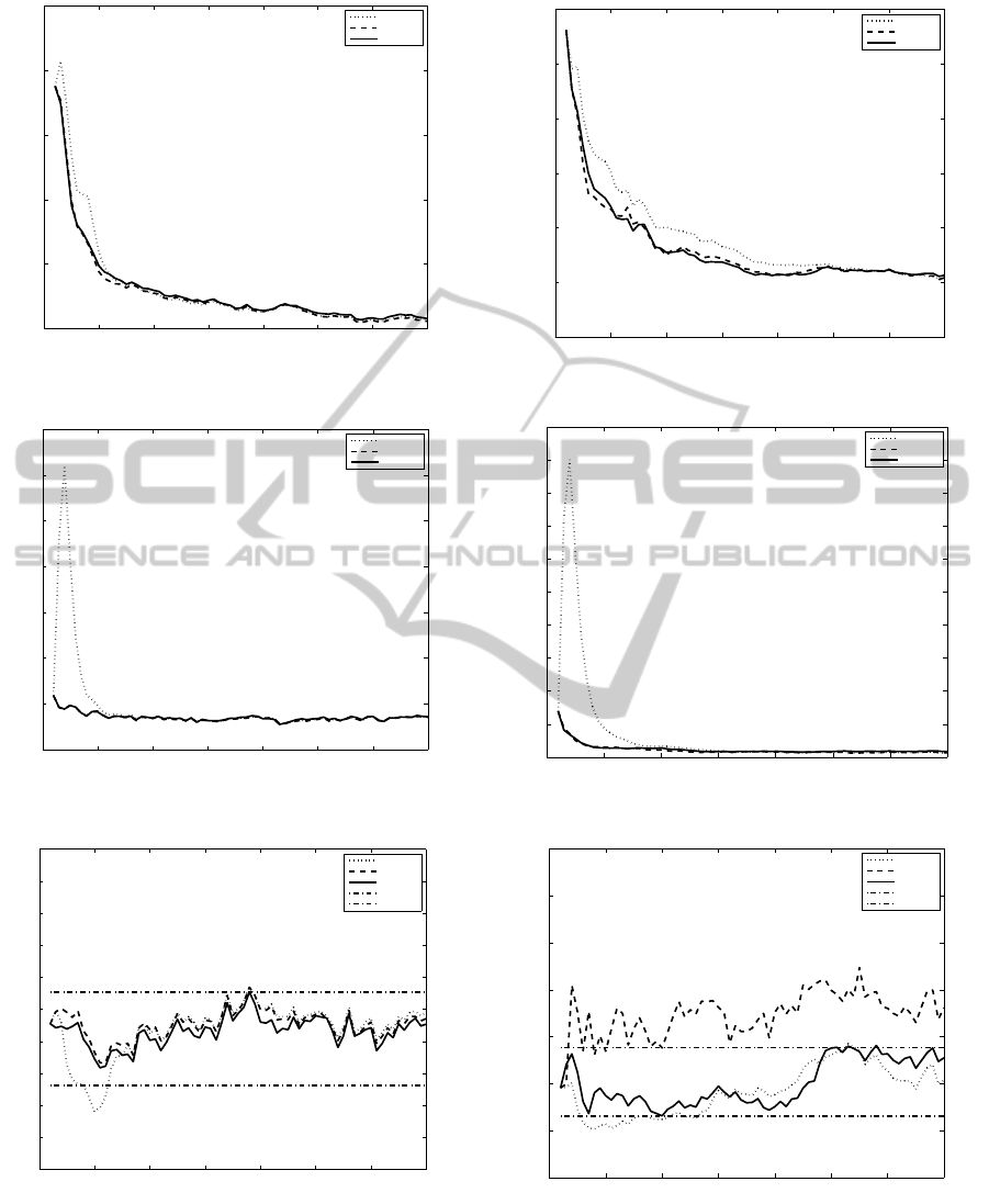
0 10 20 30 40 50 60 70

100

150

200

250

300

time (s)

RMSE in Position (m)

MCAEKF

CbGMF

GMM−ITS

(a) RMSE in position

0 10 20 30 40 50 60 70

0.2

0.4

0.6

0.8

1.2

1.4

time (s)

RMSE in Range (m)

MCAEKF

CbGMF

GMM−ITS

(b) RMSE in range

0 10 20 30 40 50 60 70

2.5

3.5

4.5

5.5

6.5

time (s)

NEES

MCAEKF

CbGMF

GMM−ITS

NEES−1

NEES−2

Figure 3: Results from the medium range scenario.

We compare the accuracy of the ﬁlters using root

mean square error (RMSE) (Bar-Shalom et al., 2001)

in position and range. The normalized (state) estima-

0 10 20 30 40 50 60 70

500

1000

1500

2000

2500

3000

time (s)

RMSE in Position (m)

MCAEKF

CbGMF

GMM−ITS

(a) RMSE in position

0 10 20 30 40 50 60 70

time (s)

RMSE in Range (m)

MCAEKF

CbGMF

GMM−ITS

(b) RMSE in range

0 10 20 30 40 50 60 70

time (s)

NEES

MCAEKF

CbGMF

GMM−ITS

NEES−1

NEES−2

Figure 4: Results from the long range scenario.

tion error squared (NEES) (Bar-Shalom et al., 2001)

can be used to determine whether a ﬁlter is consistent.

The results are presented in Figures 3-6.

ICINCO2015-12thInternationalConferenceonInformaticsinControl,AutomationandRobotics

462

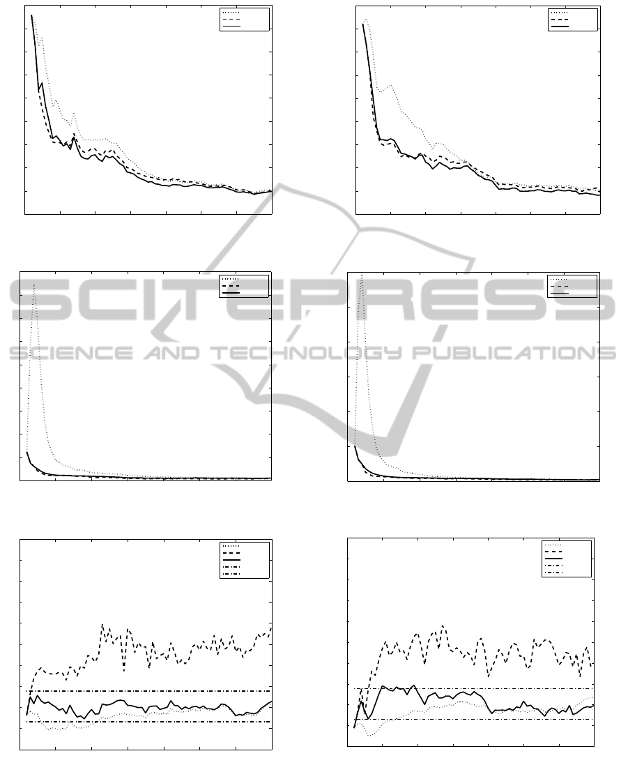
0 10 20 30 40 50 60 70

500

1000

1500

2000

2500

3000

3500

4000

4500

5000

time (s)

RMSE in Position (m)

MCAEKF

CbGMF

GMM−ITS

(a) RMSE in position

0 10 20 30 40 50 60 70

time (s)

RMSE in Range (m)

MCAEKF

CbGMF

GMM−ITS

(b) RMSE in range

0 10 20 30 40 50 60 70

time (s)

NEES

MCAEKF

CbGMF

GMM−ITS

NEES−1

NEES−2

Figure 5: Results from the very long range scenario

In scenario 1, the target is initially located at

[105, 250] km (the medium range). The GMM-ITS

divides the measurement into N = 6 components and

0 10 20 30 40 50 60 70

1000

2000

3000

4000

5000

6000

7000

8000

9000

10000

time (s)

RMSE in Position (m)

MCAEKF

CbGMF

GMM−ITS

(a) RMSE in position

0 10 20 30 40 50 60 70

time (s)

RMSE in Range (m)

MCAEKF

CbGMF

GMM−ITS

(b) RMSE in range

0 10 20 30 40 50 60 70

time (s)

NEES

MCAEKF

CbGMF

GMM−ITS

NEES−1

NEES−2

Figure 6: Results from the extremely long range scenario.

chooses α = 3 at each time k. Figures 3a, 3b and 3c

shows the performance of the MCAEKF, the CbGMF

and the GMM-ITS. These three ﬁlters have nearly the

GaussianMixtureMeasurementsforVeryLongRangeTracking

463

same position accuracy (see Figure 3a) and good con-

sistency (see Figure 3c). From Figure 3b, we can see

that both the GMM-ITS and the CbGMF have signiﬁ-

cantly smaller range errors in the early states than the

MCAEKF.

The target starts from [1050,2500] km (the long

range) in scenario 2. In the GMM-ITS, the measure-

ment likelihood is approximated by N = 12 compo-

nents with α = 3. In this scenario, as shownin Figures

4a, 4b and 4c, the GMM-ITS and the CbGMF have

obviously improved accuracy in position and range

over the MCAEKF and do not exhibit loss in range

accuracy in the early stage of ﬁltering. We can clearly

see that the GMM-ITS and the MCAEKF are consis-

tent in Figure 4c; however, in this case, the CbGMF

has a small degradation in consistency (the NEES is

around 5 instead of 4) (Tian and Bar-Shalom, 2014).

In scenario 3 and 4, the target starts much further

away from [4500,2200] km (the very long range) and

[8500,5500] km (the extremely long range), respec-

tively. Obviously, the contact lens issue is much more

of a problem than in scenario 1 and 2. In scenario

3, the parameters of the GMM-ITS are N = 24 and

α = 3.5. In order to guarantee the consistency of the

GMM-ITS, N = 48 and α = 4 are chosen in scenario

4. Figures 5a and 6a show that the GMM-ITS per-

forms better than the CbGMF and the MCAEKF in

the position RMSE. Furthermore, as shown in Figure

5c and Figure 6c, the GMM-ITS and the MCAEKF

are consistent, but the CbGMF is not.

5 CONCLUSIONS

For very long range target tracking, traditional ﬁlters

such as the EKF and the UKF are ill-equipped to solve

the contact lens problem. However, the MCAEKF

maintains consistency by using a bigger standard de-

viation of the range measurement. As a result, the

MCAEKF exhibits signiﬁcant loss in range accuracy

in the early stage of ﬁltering. The CbGMF represents

the distribution of the target state by a dynamic set

of Gaussian mixtures and can avoid the problem the

MCAEKF suffers. However, the CbGMF is consis-

tent only in the small range scenario. In the GMM-

ITS, both the measurement likelihood and the target

state pdf are approximated by a set of Gaussian mix-

tures. As shown in the simulation experiments, the

GMM-ITS is always consistent in different range sce-

narios and has small errors in positon and range. To

best of our knowledge, no other Gaussian mixture ap-

proach thus far guarantees sufﬁcient consistency and

tracking accuracy, which are crucial to ﬁlter perfor-

mance.

ACKNOWLEDGEMENTS

This work was supported by Defense Acquisition Pro-

gram Administration and Agency for Defense Devel-

opment, Korea under the contract UD140081CD.

REFERENCES

Bar-Shalom, Y., Li, X.-R., and Kirubarajan, T. (2001). Esti-

mation with Application to Tracking and Navigation.

John Wiley and Sons.

Blackman, S. and Popoli, R. (1999). Design and Analysis

of Modern Tracking Systems. Artech House.

Julier, S. J. and Uhlmann, J. K. (2004). Unscented ﬁltering

and nonlinear estimation. Proceedings of the IEEE,

92(3):401–422.

Longbin, M., Ziaoquan, S., Yiyu, Z., and Bar-Shalom, Y.

(1998). Unbiased converted measurements for track-

ing. IEEE Transactions on Aerospace and Electronic

Systems, 34(3):1023–1027.

Muˇsicki, D. (2009). Bearings only single-sensor tar-

get tracking using gaussian mixtures. Automatica,

45(9):2088–2092.

Muˇsicki, D. and Evans, R. (2006). Measurement gaussian

sum mixture target tracking. In 9th International Con-

ference on Information Fusion, Florence, Italy.

Ristic, B., Arulampalam, S., and Gordon, N. (2004). Be-

yond the Kalman Filter. Artech House.

Singer, R. A., Sea, R., and Housewright, K. B. (1974).

Derivation and evaluation of improved tracking ﬁl-

ters for use in dense multi-target environments. IEEE

Transactions on Information Theory, 20(4):423–432.

Tian, X. and Bar-Shalom, Y. (2009). Coordinate conver-

sion and tracking for very long range radars. IEEE

Transactions on Aerospace and Electronic Systems,

45(3):1073–1088.

Tian, X. and Bar-Shalom, Y. (2014). A consistency-based

gaussian mixture ﬁltering approach for the contact

lens problem. IEEE Transactions on Aerospace and

Electronic Systems, 50(3):1636–1646.

ICINCO2015-12thInternationalConferenceonInformaticsinControl,AutomationandRobotics

464