
Shaping the Current Waveform of an Active Filter for Optimized System
Level Harmonic Conditioning
Espen Skjong
1,3
, Marta Molinas
2
, Tor Arne Johansen
1
and Rune Volden
3
1
Center for Autonomous Marine Operations and Systems, Department of Engineering Cybernetics, Norwegian University
of Science and Technology, Trondheim, Norway
2
Department of Engineering Cybernetics, Norwegian University of Science and Technology, Trondheim, Norway
3
Ulstein Power & Control AS, Ulsteinvik, Norway
Keywords:
System Level Harmonic Conditioning, Model Predictive Control, Active Filter (AF), Multiple Shooting,
Non-linear Loads, Total Harmonic Distortion (THD).
Abstract:
Harmonic voltages and currents in electrical systems, when present to a certain degree, represent not only a
power quality problem but they are also strongly associated with the electrical system overall losses and they
are arguably a source of instability and a safety concern. Mitigating harmonics distortion across the entire
system by actively reducing harmonic currents propagation is an effective way of coping with these issues and
can be dealt with the injection of a compensating current waveform with an active filter installed at a given
bus. This paper shows how, by shaping the compensating current waveform in an optimal way, the overall
electrical system harmonic distortion can be optimally reduced in a cost effective manner with a minimum
size of the compensating device. The process of shaping this optimal compensating current is shown by how
its components are defined by the optimization algorithm using the phase and amplitude of each harmonic as
degrees of freedom in the process of finding the optimal waveform. A marine vessel distribution grid is used
as representative example to prove the concept.
1 INTRODUCTION
Pure, continuous and constant frequency sinusoidal
waveforms are the ideal waveforms in most electric
power systems. A given deviation from this ideality
is defined as a power quality issue and limits of toler-
ance are adopted by various standards. Harmonic dis-
tortion is one of the possible forms of deviation from
a pure sinusoidal waveform. Harmonic distortion is
a stationary form of distortion caused by the pres-
ence of additional sinusoidal components or harmon-
ics components at multiples of the fundamental fre-
quency component carrying the electrical signal un-
der consideration. Most common sources of these dis-
tortions are non-linear loads such as multi (6, 12, 18,
24)-pulse rectifiers, line-commutated converters, high
frequency harmonics from voltage source converters
(VSC) and switch mode power supplies, saturated
transformers and other magnetic components, and
power system background voltage distortions (Akagi
et al., 2007). These non-linear loads will generally
draw a distorted current containing several harmonic
components that are multiples of the fundamental fre-
quency component. With a sinusoidal voltage at the
source, these harmonic currents will not carry active
power to the load but will be circulating as reactive
currents in the distribution system and will represent
extra distribution losses. One way of approaching this
problem is to over-dimension the system to be able
to stand the side effects of these harmonics by de-
sign. For achieving that, generation, distribution sys-
tems and loads will need to be designed over-rated to
cope with vibration (generators, motors, transform-
ers), heating and losses originated by these harmonic
currents circulating in the system (Evans et al., 2007).
This measure however will not alleviate the inher-
ent power quality issues associated with the presence
of harmonics which will be reflected at the end-user
side. Stability issues in electrical networks have also
been correlated with the presence of harmonics (Bing
et al., 2007) and reduced stability margins have been
reported in association with that. The requirements
of power quality standards and safety in electrical in-
stallations demand the use of a more active approach
when coping with harmonics. Such approach should
be aimed at actively reducing the impact of harmonics
98
Skjong E., Molinas M., Johansen T. and Volden R..
Shaping the Current Waveform of an Active Filter for Optimized System Level Harmonic Conditioning.
DOI: 10.5220/0005488800980106
In Proceedings of the 1st International Conference on Vehicle Technology and Intelligent Transport Systems (VEHITS-2015), pages 98-106
ISBN: 978-989-758-109-0
Copyright
c
2015 SCITEPRESS (Science and Technology Publications, Lda.)

on power quality by minimizing the total harmonics
distortion (THD) using passive or active harmonic fil-
tering techniques. Actively filtering or mitigating the
harmonics will have direct implications not only in
the quality of the electricity delivered but also in fuel
savings, revenues for power transactions, investments
in installed capacity of electrical system components,
efficient utilization of existing installations and reduc-
tion of overall system losses.
Mitigation of harmonics in electrical systems with
dispersed generation and loads can be approached by
finding the optimum shape of the current wave form
that an active filter should inject in a given bus in or-
der to minimize the propagation of harmonics in the
entire electrical system. This paper, with references to
(Skjong et al., 2015a) and (Skjong et al., 2015b), pro-
poses such an approach based on optimization where
the objective is to search for the optimum shape of the
current waveform to be injected by an active filter to
minimize the THD of the entire electrical system. To
prove the concept, the optimization algorithm is im-
plemented in the electrical system of a marine vessel
(a discussion of harmonic mitigation using an active
filter in a marine vessel’s power distribution grid is
given in (Rygg Aardal et al., 2015)). The benefits of
a system level harmonic mitigation approach is com-
pared with the classical approach of local active fil-
tering. The current waveform shaping process and
components resulting from the optimization search
are shown for two different loading examples. The
component waveforms of the compensating current
clearly shows how the optimization algorithm effec-
tively exploits the amplitude and phases of each har-
monic component when searching for the optimum
waveform shape. A major finding from this research
is the possibility to minimize not only the THD of the
entire system but to achieve that with the minimum
required current rating of the active filter. This will in
turn have implications in reducing the investment in
the compensating device.
2 POWER DISTRIBUTION GRID
MODEL
Power electronics has become the most essential part
in modern electrical distribution systems as coupling
element between generation, loads and the electri-
cal network as they provide flexibility and fast con-
trol capabilities. Most recently, with the emergence
of the smartgrid, and due to its inherent properties
of fast actuation capabilities and extreme flexibility,
power electronics will be critical in the realization
of smart grid systems and microgrids which require
different voltage levels conversion, frequency conver-
sion capabilities, real-time supply-load match and hy-
brid AC/DC and DC/AC couplings. Representative
examples of these systems are onshore and offshore
wind farms connected to a national power distribution
network where power electronics in the form of Volt-
age Source Converters (VSC), High Voltage Direct
Current (HVDC) systems, Active Filters (AF), Solid
State Transformers (SST), etc., are critical for collect-
ing and distributing the generated power in defined
voltage levels and within quality standards. Stand-
alone electrical grids are another example in which
power electronics play an essential role in enabling
the operation and control of such systems. A stand-
alone microgrid, a wave energy generation plant, an
isolated PV generation system and a marine vessel’s
power distribution grid (Patel, 2011) are typical ex-
amples with multiple and dispersed power genera-
tion units, e.g. diesel engines, gas turbines, fuel cells
and batteries, generating the power needed for dif-
ferent operation scenarios. Despite its enormous ad-
vantages, power electronics introduce new non-linear
properties and due to its switching mode of operation,
it constitutes a source of harmonic distortion in the
systems in which they are operating.
>ŽĂĚϭ
ϭ
>
^ϭ
>
D
ŝ
>ϭ
ŝ
D
ŝ
>Ϯ
ŝ
&
,ĂƌŵŽŶŝĐ
&ŝůƚĞƌ
ŝ
ϭ
ŝ
^ϭ
Ͳ
ǀ
ϭ
н
ǀ
^ϭ
Ͳǀ
>Dн
Ͳ
ǀ
>^ϭ
н
Ϯ
ŝ
Ϯ
Ͳ
ǀ
Ϯ
н
>
^Ϯ
ŝ
^Ϯ
ǀ
^Ϯ
Ͳ
ǀ
>^Ϯ
н
^ŽƵƌĐĞϮ
Z
^ϭ
Z
D
Z
^Ϯ
>ŽĂĚϮ
^ŽƵƌĐĞϭ
DĂŝŶƵƐ
ƵƌƌĞŶƚŵĞĂƐƵƌĞŵĞŶƚƐ
Figure 1: Simplified model of an AC power distribution
grid.
In this work a simplified stand-alone power dis-
tribution grid is assumed. The power grid, shown in
figure 1 with details given in table 1, connects two
power sources to two non-linear loads and can resem-
ble a simplified marine vessel microgrid. The loads
which can represent the propulsion system are taken
as the sources of harmonic pollution in this study. A
6-pulse diode rectifier is considered to be part of the
drive system and the harmonic pollution is modelled
accordingly. An active harmonic filter based on a
ShapingtheCurrentWaveformofanActiveFilterforOptimizedSystemLevelHarmonicConditioning
99

Table 1: Power distribution grid parameters used in case
study.
Parameter
Value
L
S1
1 mH
L
S2
1 mH
L
MB
1 mH
R
S1
(0.1·L
S1
·ω) Ω
R
S2
(0.1·L
S2
·ω) Ω
R
MB
(0.1·L
MB
·ω) Ω
C
1
0.1 µF
C
2
0.1 µF
voltage source converter connected to one of the load
buses is considered for injecting a compensating cur-
rent which will be shaped by the optimization algo-
rithm for the purpose of system level harmonic miti-
gation.
2.1 Model Formulation
Considering figure 1 and using Kirchhoff’s laws a set
of differential equations describing the grid’s physical
behavior can be derived,
L
S1
di
S1
dt
= v
S1
−R
S1
i
S1
−v
C1
C
1
dv
C1
dt
= i
S1
−i
MB
−i
L1
L
MB
di
MB
dt
= v
C1
−v
C2
−R
MB
i
MB
C
2
dv
C2
dt
= i
MB
+ i
S2
−i
L2
+ i
F
L
S2
di
S2
dt
= v
S2
−R
S2
i
S2
−v
C2
.
(1)
The generators are modeled as ideal voltage sources
with a voltage phase shift φ
V
,
v
S
(t) =
√
2V
rms
sin(ωt + φ
V
), (2)
while the non-linear loads are modeled as current
sources with harmonic components of order 5,7,11
and 13 with phase shifts φ
L,i
and peak values (am-
plitudes) I
L,i
,
i
L
(t) =
∑
i
I
L,i
sin
i
ωt + φ
L,i
,
∀i ∈{1, 6k±1|k = 1, 2}.
(3)
The harmonic filter is designed to suppress harmonic
pollution and can be modeled as a current source with
harmonic components of order 5, 7, 11 and 13,
i
F
(t) =
∑
i
I
F,i
sin
i
ωt + φ
F,i
,
∀i ∈{6k ±1|k = 1, 2},
(4)
where I
F,i
is the peak values (amplitudes) of the fil-
ter’s harmonic current component i. The grid model
stated above is given as a single phase configuration.
A single phase configuration is not a realistic config-
uration in microgrids, and the equations given above
should be extended to a three-phase configuration.
2.2 Three-phase Three-wire
Configuration
Three-phase configurations could consist of three or
four wires. The three-phase configuration is modeled
using the Clarke transform (Akagi et al., 2007), which
converts the abc phases to αβ0 phases. Assuming bal-
anced sources the neutral wire (fourth wire) is exces-
sive and the αβ0 frame is simplified to αβ, where the
β current is lagging the α current by 90
◦
. Hence, in
this work a three-phase three-wire configuration is as-
sumed.
The three-phase three-wire αβ form is derived by
extending the single-phase model to three-phase abc
form. The abc form is then transformed to αβ us-
ing the Clarke transformation. As an example, the
three-phase three-wire model for the voltage sources,
assuming balanced sources, can be written in the αβ
frame as
v
S
(t) =
v
S,α
(t)
v
S,β
(t)
=
√
3V
rms
sin(ωt + φ
V
)
√
3V
rms
sin(ωt + φ
V
+
π
2
)
. (5)
In the same way the load and filter models are ex-
tended to three-phase three-wire using the αβ frame,
however, the phase shifts φ
L,i
and φ
F,i
for the filter
model and the load models should be equal for the α
and β phases due to the definition of the β phase lag-
ging the α phase by 90
◦
. Also the filter amplitudes in
the αβ frame are kept equal for each harmonic com-
ponent when considering balanced loads to ensure a
balanced filter.
In the rest of this paper subscript α and β are used
to denote the α and β phases for each voltage and
current component, and the vectors (phasors) v and
i are used to represents voltages and currents, respec-
tively, given in the αβ frame. It is referred to (Ak-
agi et al., 2007) for details regarding the αβ frame in
three-phase three-wire configurations.
2.3 Active Filter (AF) Constraints
The harmonic filter model is constrained due to phys-
ical limitations of an active filter. The active filter’s
switching circuit (IGBTs) in conjunction with the rat-
ing of the voltage controlled capacitor, decides the ac-
tive filter’s power rating. The IGBT will be the crucial
component deciding the filter’s current rating, formu-
lated as current limits in the abc phases. Figure 2 il-
lustrates the active filter’s current limits in both the
VEHITS2015-InternationalConferenceonVehicleTechnologyandIntelligentTransportSystems
100

i
α
i
β
i
a
i
c
i
b
i
lim
F
i
ap
F
i
min
b
i
max
c
i
min
c
i
max
b
i
min
a
i
max
a
Current phasor
limitations
Phase current
limitations
30
◦
120
◦
Figure 2: Harmonic filter constraints: Three-phase three-
wire represented by the αβ and abc frames (Suul, 2012).
abc and the αβ frames. In the abc frame the phases
are restricted by
i
min
j
≤ i
j
≤i
max
j
, ∀j ∈ {a, b, c}, (6)
which forms the hexagon given in figure 2. These
restrictions can be expressed in the αβ frame by
−i
lim
F
≤ −i
F,β
+
√
3
3
i
F,α
≤i
lim
F
(7a)
−i
lim
F
≤ i
F,β
+
√
3
3
i
F,α
≤i
lim
F
(7b)
−i
ap
F
≤ i
F,α
≤i
ap
F
(7c)
−i
lim
F
≤ i
F,β
≤ i
lim
F
, (7d)
where the hexagon’s apothem is given by
i
ap
F
=
√
3
2
i
lim
F
,
(8)
and i
lim
F
is a design variable representing the filter’s
phase current limitations. Eq. (7) gives a set of lin-
ear constraints which will be used in an optimization
scheme to conduct as much harmonic conditioning as
possible for the given power rating. For notational
simplicity we define the feasible region for the filter’s
current vector i
F
∈ S.
3 MODEL PREDICTIVE
CONTROL
Using the power grid model derived in the previ-
ous section an optimization procedure is developed
to minimize, by control, the total harmonic currents
in the power grid, and prevent harmonic distortions
from propagating from the loads to the sources. The
optimization procedure is stated as a non-linear model
predictive control (NMPC) (Rawlings and Mayne,
2009).
3.1 Formulating the Power Grid Model
in Standard NMPC Form
A NMPC problem for the filter current reference gen-
eration in standard form can be stated as
min
p,u
V(x, z, u, p) =
N
∑
n=1
l(x
n
, z
n
, u
n−1
, p)
s.t.
˙
x
n
= f(x
n
, z
n
, u
n−1
, p) ∀n ∈ {1, . . . , N}
g(x
n
, z
n
, u
n−1
, p) = 0, ∀ n ∈ {1, . . . , N}
h(x
n
, z
n
, u
n−1
, p) ≤ 0|i
F,n
∈ S, ∀n ∈ {1, . . . , N}
given initial values x
0
, z
0
|initial value i
F,0
∈ S,
(9)
where the objective function V(·) and the stage cost
function l(·) defines the goal of the optimization. In-
dex n is the time step in the control horizon. The vec-
tors x, z, u and p defines the dynamic states, the al-
gebraic states, the controls and the parameters of the
problem formulation, respectively. g(·) represents the
problem’s equality constraints while h(·) represents
the inequality constraints. Assuming that higher or-
der harmonics (5th, 7th, 11th and 13th) generated by
a 6-pulse diode rectifier are known and given by
i
hh
L
=
∑
i
I
L,α,i
sin
i
ωt +φ
L,i
∑
i
I
L,β,i
sin
i
ωt + φ
L,i
+
π
2
,
∀i ∈ {6k±1|k = 1, 2},
(10)
the algebraic state vector can be stated as
z =
h
v
⊤
S1
, v
⊤
S2
, i
⊤
L1
, i
⊤
L2
, i
⊤
F
, (i
hh
L1
)
⊤
, (i
hh
L2
)
⊤
i
⊤
,
(11)
where the loads i
L1
and i
L2
are the three-phase three-
wire extension of eq. (3) given in the αβ frame, the
filter currenti
F
is the three-phase three-wire extension
of eq. (4) given in the αβ frame, and the harmonic
components of each load, i
hh
L1
and i
hh
L2
, are given by eq.
(10). The dynamic state vector is given by the power
grid model’s differential states,
x =
h
i
⊤
S1
, i
⊤
S2
, i
⊤
MB
, v
⊤
C1
, v
⊤
C2
i
⊤
.
(12)
The control vector, often referred to as manipulated
variables, consists of the active filter’s amplitude and
phase components,
u =
I
F,α,i
, I
F,β,i
, φ
F,i
⊤
, ∀i ∈{6k ±1|k = 1, 2}
(13)
and the parameter vector is given by p = 0. The
stage cost function, which should be a convex func-
tion, addresses the goal of the optimization, which in
ShapingtheCurrentWaveformofanActiveFilterforOptimizedSystemLevelHarmonicConditioning
101

this work is to minimize the harmonic pollution in the
power grid. A suitable stage cost function is given as
l(x, z, u, p) = q
1
i
F,α
−i
hh
L1,α
2
+ q
1
i
F,β
−i
hh
L1,β
2
+ q
2
i
F,α
−i
hh
L2,α
2
+ q
2
i
F,β
−i
hh
L2,β
2
+ q
u
u
⊤
I
F
u
I
F
,
(14)
with constant weights q
1
, q
2
, q
u
, where u
I
F
⊂ u that
includes the filter’s amplitudes. The last part in eq.
(14) is added to minimize the filter amplitudes, hence
minimizing the filter’s power rating, and also provid-
ing stability and robustness with regards to modeling
errors. q
u
< q
1
, q
2
as minimizing the power rating
is of lesser importance than decreasing the harmonic
distortion in the power grid.
4 RESULTS
The main objectiveof this work is to use the NMPC to
generate optimized active filter current references by
considering the harmonic pollution from both loads
and utilizing filter current amplitudes and phases as
control variables. Two case studies are proposed, one
with symmetric and one with asymmetric loads. In
both cases the loads introduce a high level of har-
monic pollution in form of the 5th, 7th, 11th and 13th
harmonic components, and the active filter currents
are limited to i
lim
F
= 0.5 [pu] (i
ap
F
=
√
3
4
[pu]). The
load currents for both study cases are presented in ta-
ble 2. A local filter reference generation (local filter-
ing) considering only load 2 is implemented for com-
parison purposes. It is important to remark that the
local filtering does not consider the filter’s physical
limits and generates filter currents exactly mimicking
the harmonic currents from load 2 with a phase shift
of 180
◦
. The fundamental frequencyis fixed to f = 50
[Hz] in both study cases.
4.1 Symmetric Loads
Figure 3 and 4 represents the simulation results for
case 1 in table 2. The upper plot in figure 3(a) repre-
sents the NMPC filter current and local filtering cur-
rent in the a phase. The local filtering current is the
saturated load 2 harmonics phase shifted 180
◦
. By
comparing the two filter currents one clearly see that
the NMPC filter current has different amplitudes from
the local filtering current, and at approximated time
instances 0.0025 and 0.0175 [s], among others, the
NMPC filter current’s phases (one phase for each har-
monic component)have been altered, which is seen as
a deviation from the local filter current’s visual repre-
sentation.
The four lower plots in figure 3(a) represent the
load voltages (a phase) and respective frequency
spectra’s with calculated THD values. Due to numer-
ical errors related to discretization, the THD values
are calculated based on a frequency spectrum in a
range of 0-650 [Hz]. With either filtering technique
the THD of load 2 voltage is lower than load 1. This
is as expected since the active filter is installed near
load 2. Hence the load 1 voltage will in either case
be more distorted than the load 2 voltage due to the
inductance in the main bus preventing the filter to per-
fectly compensate for all the harmonics generated by
load 1 and 2. As can be seen, the THD values from
local filtering is higher compared to the NMPC case.
First of all, the local filtering does not take into con-
sideration the filter’s limitation and load 1 harmonics,
and the compensating filter current using this filtering
technique would be the 180
◦
phase shifted load 2 har-
monics. However, the filter is too small to cope with
the distorted grid, which means the filter will saturate
the calculated filter current references from local fil-
tering resulting in a THD value for load 1 almost as
high as without filtering (19.5%). The NMPC, how-
ever, takes into account both loads and also the filter
limits in the calculation of optimal filter current refer-
ences. This way the filter current references will not
be saturated due to exceeding the active filter’s phys-
ical limits.
Figure 3(b) represents the filter current (phase a)
frequency spectra for both NMPC and local filter-
ing. As can be seen, the amplitudes for the domi-
nant frequency components are generally lower for
the NMPC filter current than for the local filtering cur-
rent. The filter current were modeled by the 5th, 7th,
11th and 13th harmonic component, which represents
frequencies of 250, 350, 550 and 650 [Hz]. As evi-
dent from the plot, other frequency components are
utilized by the NMPC due to the ability to rapidly
manipulate the harmonic components’ phases. Due
to the saturation of the local filtering current other
harmonic components than those modeled are also
present in the frequency spectra.
Figure 4 represents the 5th, 7th, 11th and 13th har-
monic components of the NMPC filter current and lo-
cal filtering current in the a phase. From this rep-
resentation it is easy to show that the NMPC does
utilize both, the amplitudes and the phases of each
modeled harmonic component in the filter reference
current. The load 2 current, which also represents
the unsaturated reference current from local filtering,
and the NMPC do share the same fundamental fre-
quency, but due to the utilization of the harmonic
VEHITS2015-InternationalConferenceonVehicleTechnologyandIntelligentTransportSystems
102
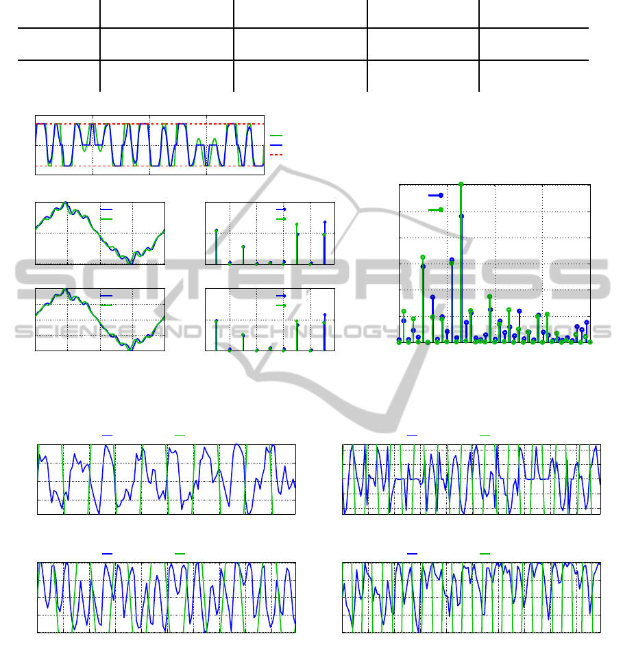
Table 2: Study case configurations.
Load 1 amplitudes Load 2 amplitudes Load 1 phases Load 2 phases
[1th, 5th, 7th, 11th, 13th] [1th, 5th, 7th, 11th, 13th] [1th, 5th, 7th, 11th, 13th] [1th, 5th, 7th,11th, 13th]
Case 1 I
α
L1
= I
β
L1
I
α
L2
= I
β
L2
φ
L1
= [0, 0, 0, 0, 0] φ
L2
= [0, 0, 0, 0, 0]
(symmetric)
= [0.9, 0.6, 0.3, 0.5, 0.8] = [0.9, 0.6, 0.3, 0.5, 0.8]
Case 2 I
α
L1
= I
β
L1
I
α
L2
= I
β
L2
φ
L1
= [0, 0, 0, 0, 0] φ
L2
= [0, 0, 0, 0, 0]
(asymmetric)
= [0.9, 0.8, 0.6, 0, 0.5] = [0.9, 0, 0.6, 0.8, 0]
0 0.005 0.01 0.015 0.02
−0.5
0
0.5
Time [s]
i
F
a
[pu]
Local filtering
NMPC
Filter limits
0 0.005 0.01 0.015 0.02
−1
0
1
Time [s]
v
L1
a
[pu]
NMPC
Local filtering
300 400 500 600
0
0.05
0.1
Frequency [Hz]
|v
L1
a
|
THD:15.7%
THD:18.2%
0 0.005 0.01 0.015 0.02
−0.5
0
0.5
Time [s]
v
L2
a
[pu]
NMPC
Local filtering
300 400 500 600
0
0.05
0.1
Frequency [Hz]
|v
L2
a
|
THD:14.4%
THD:15.6%
(a) Filter currents and load voltages.
0 500 1000 1500 2000
0
0.05
0.1
0.15
0.2
0.25
0.3
Frequency [Hz]
|i
F
a
|
NMPC filter current
Local filtering filter current
(b) Filter current spectrum.
Figure 3: Case 1 (symmetric loads): Filter currents and filtered load voltages.
0 0.002 0.004 0.006 0.008 0.01 0.012 0.014 0.016 0.018
−0.05
0
0.05
0.1
Time [s]
i
5
a
[pu]
NMPC filter current
Load 2 current
0 0.002 0.004 0.006 0.008 0.01 0.012 0.014 0.016 0.018
−0.1
−0.05
0
0.05
0.1
Time [s]
i
7
a
[pu]
NMPC filter current
Load 2 current
(a) 5th and 7th filter current component.
0 0.002 0.004 0.006 0.008 0.01 0.012 0.014 0.016 0.018
−0.1
−0.05
0
0.05
0.1
Time [s]
i
11
a
[pu]
NMPC filter current
Load 2 current
0 0.002 0.004 0.006 0.008 0.01 0.012 0.014 0.016 0.018
−0.1
−0.05
0
0.05
0.1
Time [s]
i
13
a
[pu]
NMPC filter current
Load 2 current
(b) 11th and 13th filter current component.
Figure 4: Case 1 (symmetric loads): Filter current components.
phases the NMPC filter current components are com-
pletely changed and it is not easy to determine neither
frequency nor period from the plots. One important
finding is the total magnitude of each harmonic fil-
ter current component. As can be seen, the filter cur-
rent components, in this case, do not increase beyond
0.12 [pu]. Compared to the local filtering, utilization
of filter current phases would be an important degree
of freedom when coping with high harmonic pollu-
tions using a relative small active filter. Active filters
are generally quite expensive, thus increasing the fil-
ter size could be a costly affair.
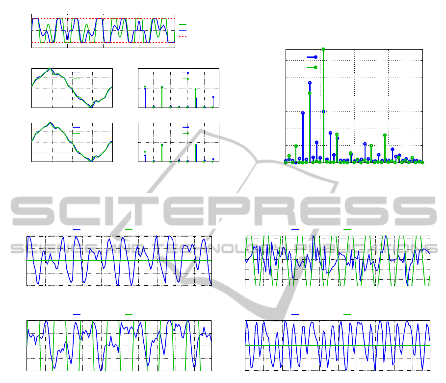
4.2 Asymmetric Loads
Figure 5 and 6 represents the simulation results for
case 2 in table 2. The upper plot in figure 5(a), as
in the previous case, represents the NMPC filter cur-
ShapingtheCurrentWaveformofanActiveFilterforOptimizedSystemLevelHarmonicConditioning
103
0 0.005 0.01 0.015 0.02
−0.5
0
0.5
Time [s]
i
F
a
[pu]
Local filtering
NMPC
Filter limits
0 0.005 0.01 0.015 0.02
−0.5
0
0.5
Time [s]
v
L1
a
[pu]
NMPC
Local filtering
300 400 500 600
0
0.05
0.1
Frequency [Hz]
|v
L1
a
|
THD:14.6%
THD:18.6%
0 0.005 0.01 0.015 0.02
−0.5
0
0.5
Time [s]
v
L2
a
[pu]
NMPC
Local filtering
300 400 500 600
0
0.05
0.1
Frequency [Hz]
|v
L2
a
|
THD:12.6%
THD:14.1%
(a) Filter currents and load voltages.
0 500 1000 1500 2000
0
0.05
0.1
0.15
0.2
0.25
0.3
Frequency [Hz]
|i
F
a
|
NMPC filter current
Local filtering filter current
(b) Filter current spectrum.
Figure 5: Case 2 (asymmetric loads): Filter currents and filtered load voltages.
0 0.002 0.004 0.006 0.008 0.01 0.012 0.014 0.016 0.018
−0.1
−0.05
0
0.05
0.1
Time [s]
i
5
a
[pu]
NMPC filter current
Load 2 current
0 0.002 0.004 0.006 0.008 0.01 0.012 0.014 0.016 0.018
−0.05
0
0.05
0.1
Time [s]
i
7
a
[pu]
NMPC filter current
Load 2 current
(a) 5th and 7th filter current component.
0 0.002 0.004 0.006 0.008 0.01 0.012 0.014 0.016 0.018
−0.4
−0.2
0
0.2
0.4
Time [s]
i
11
a
[pu]
NMPC filter current
Load 2 current
0 0.002 0.004 0.006 0.008 0.01 0.012 0.014 0.016 0.018
−0.1
−0.05
0
0.05
0.1
Time [s]
i
13
a
[pu]
NMPC filter current
Load 2 current
(b) 11th and 13th filter current component.
Figure 6: Case 2 (asymmetric loads): Filter current components.
rent and the local fingering current in the a phase.
In this case the NMPC filter current is more phase
shifted, compared to the local filtering current, than
in the synchronous loads case. This is a direct con-
sequence of the optimization trying to condition both
load currents. The phase shifting, compared to local
filtering, is illustrated at, among others, approximated
time instances 0.002 and 0.008 [s].
The four lower plots in figure 5(a) shows that the
differences in THD for NMPC and local filtering are
higher in the asymmetric case than in the symmet-
ric case. This is due to the NMPC’s consideration of
all loads, whereas local filtering does only consider
load 2. Also, the filter limits saturate the local filter
currents, as pointed out in the previous case, prevent-
ing the filter from conducting the intended filtration.
Compared with no filtering for v
L1
(21.1%) the lo-
cal filtering approach performs poorly. The NMPC
avoids filter current saturation by considering the fil-
ter limits and by utilizing the filter current amplitudes
and phases to make the best possible harmonic condi-
tioning out of the filter.
Figure 5(b) showcases the filter current (phase a)
frequency spectra for both NMPC and local filtering.
The discussion and analysis from the symmetric case
is also applicable for the asymmetric case. In general,
dominant current amplitudes are smaller in the case of
NMPC than for local filtering. However, the NMPC
utilizes the filter current phases to utilize un-modeled
frequency components with its cause of lowering the
filter current amplitude. This is seen in the figure
where amplitudes of the frequency components, apart
from the 5th, 7th, 11th and 13th, are generally higher
for the NMPC case than for local filtering. Due to the
VEHITS2015-InternationalConferenceonVehicleTechnologyandIntelligentTransportSystems
104

configuration of the asymmetric loads, which for the
loads combined includes all modeled frequency com-
ponents, the NMPC will represent harmonic compo-
nents present in both loads. This can be seen in the
5th component (250 [Hz]), whereas the NMPC has
a non-zero amplitude compared with the local filter-
ing’s zero amplitude.
The 5th, 7th, 11th and 13th harmonic components
of the NMPC’s filter current in phase a are showcased
in figure 6 compared with the load 2 current in the
same phase. As can be seen from the configuration in
table 2 and from the figure, the 5th and 13th harmonic
component in load 2 are zero. However, due to asym-
metric loads all NMPC filter current components are
utilized. This is due to the fact that load 1 and 2 com-
bined represents all modeled harmonics polluting the
grid. As with the symmetric case, the NMPC filter
current components are non-periodic due to the rapid
utilization of the filter amplitudes and phases for each
harmonic component. As a result of rapidly altering
the phases and amplitudes for each harmonic compo-
nent, the amplitudes can be kept small, which is illus-
trated in figure 6 where none of the filter components
reach a higher amplitude than 0.1 [pu]. As a result of
the utilization of amplitudes and phases for each mod-
eled harmonic component, the NMPC could also pre-
vent un-modeled harmonics from polluting the grid.
This is a useful property specially when simple grid
models are available for a real-time implementation
of the optimization scheme.
5 CONCLUSIONS
A non-linear model predictive controller (NMPC) ap-
plied to system level harmonic conditioning in a gen-
eralized power grid has been outlined and discussed
in detail. Two different study cases were presented.
A local filtering procedure was introduced to compare
with the NMPC filter reference current generation ap-
proach and to highlight the benefits of system level
harmonics mitigation.
The NMPC was able to achieve better harmonic
conditioning than the local filtering due to the consid-
eration of both loads and the active filter’s physical
limits. The NMPC’s ability to rapidly alter the am-
plitudes and phases of each modeled harmonic com-
ponents in the filter current gave flexibility in terms
of un-modeled harmonic components present in the
loads, the ability to optimize the harmonic mitiga-
tion with limited filter’s size and distortions from both
loads. The NMPC’s ability to alter the phases and
amplitudes of each harmonic filter current component
is important when un-modeled harmonic frequency
components are present in the loads, and a simple
power grid model could be enough to obtain a real-
time implementation of the NMPC. Compared with
the local filtering, the NMPC was not affected by sat-
uration of the filter current references. The saturation
of the local filtering resulted in higher THDs. With
the system level harmonics mitigation approach, the
NMPC was able to optimize the active filter current
to achieve the best possible harmonic conditioning for
both load currents with a given filter’s physical limi-
tations.
ACKNOWLEDGEMENT
This work has been carried out at the Centre for Au-
tonomous Marine Operations and Systems (AMOS),
supported by Ulstein Power & Control AS and
The Norwegian Research Council, project number
241205.
REFERENCES
Akagi, H., Watanabe, E., and Aredes, M. (2007). Instanta-
neous Power Theory and Applications to Power Con-
ditioning. IEEE Press Series on Power Engineering.
Wiley.
Bing, Z., Karimi, K., and Sun, J. (2007). Input impedance
modeling and analysis of line-commutated rectifiers.
In IEEE Power Electronics Specialists Conference,
2007. PESC 2007, pages 1981–1987.
Evans, I., Hoevenaars, A., and Eng, P. (2007). Meeting har-
monic limits on marine vessels. In Electric Ship Tech-
nologies Symposium, 2007. ESTS ’07. IEEE, pages
115–121.
Patel, M. (2011). Shipboard Electrical Power Systems.
Shipboard Electrical Power Systems. Taylor & Fran-
cis.
Rawlings, J. and Mayne, D. (2009). Model Predictive Con-
trol: Theory and Design. Nob Hill Pub.
Rygg Aardal, A., Skjong, E., and Molinas, M. (2015). Han-
dling system harmonic propagation in a diesel-electric
ship with an active filter. In ESARS 2015 Confer-
ence on Electrical Systems for Aircraft, Raukway, Ship
Propulsion and Road Vehicles.
Skjong, E., Molinas, M., and Johansen, T. A. (2015a). Op-
timized current reference generation for system-level
harmonic mitigation in a diesel-electric ship using
non-linear model predictive control. In IEEE 2015
International Conference on Industrial Technology,
ICIT.
Skjong, E., Ochoa-Gimenez, M., Molinas, M., and Jo-
hansen, T. A. (2015b). Management of harmonic
propagation in a marine vessel by use of optimiza-
tion. In IEEE Transportation Electrification Confer-
ence and Expo 2015 (ITEC).
ShapingtheCurrentWaveformofanActiveFilterforOptimizedSystemLevelHarmonicConditioning
105

Suul, J. A. (2012). Control of Grid Integrated Volt-
age Source Converters under Unbalanced Conditions.
PhD thesis, Norwegian University of Science and
Technology, Department of Electrical Power Engi-
neering.
VEHITS2015-InternationalConferenceonVehicleTechnologyandIntelligentTransportSystems
106
