Gramophone Noise Reconstruction

A Comparative Study of Interpolation Algorithms for Noise Reduction

Christoph F. Stallmann and Andries P. Engelbrecht

Department of Computer Science, University of Pretoria, Pretoria, South Africa

Keywords:

Gramophone Records, Interpolation, Audio Reconstruction, Polynomials, Signal Modelling.

Abstract:

Gramophone records have been the main recording medium for seven decades and regained widespread pop-

ularity over the past few years. Records are susceptible to noise caused by scratches and other mishandlings,

often making the listening experience unpleasant. This paper analyses and compares twenty different inter-

polation algorithms for the reconstruction of noisy samples, categorized into duplication and trigonometric

approaches, polynomials and time series models. A dataset of 800 songs divided amongst eight different gen-

res were used to benchmark the algorithms. It was found that the ARMA model performs best over all genres.

Cosine interpolation has the lowest computational time, with the AR model achieving the most effective inter-

polation for a limited time span. It was also found that less volatile genres such as classical, country, rock and

jazz music is easier to reconstruct than more unstable electronic, metal, pop and reggae audio signals.

1 INTRODUCTION

Gramophone records were the ﬁrst commercial audio

storage medium with the introduction of Berliner’s

turntable in 1889 (Wile, 1990). Records continued

to be widely used for more than seven decades, un-

til they were replaced by the compact disc (CD) in

the late 1980s. Although downloadable digital music

has become the forerunner in the 20

century, gramo-

phone sales have surged in the past few years, achiev-

ing record sales since they were discontinued as main

music medium in 1993. Approximately six million

records were sold in the United States alone in 2013,

an increase of 33% from the previous year (Richter,

2014). However, the Nielsen Company indicated that

only 15% of the sales were logged, since most gramo-

phone records do not have a bar code which is used to

track sales (CMU, 2011). Besides an increase in sales

of new records, most recordings prior to the 1960s are

only available on gramophone. Efforts are made by

both commercial music labels and private audiophiles

to digitize these historic records. The digitization pro-

cess is a tedious and time consuming process, since

most records are damaged and need to be refurbished.

This paper examines twenty different interpola-

tion algorithms that are utilized for the digital restora-

tion of audio signals that are distorted by scratches

and other physical damage to the record. This re-

search is part of a larger project aimed at automating

the detection and reconstruction of noise on damaged

gramophone records, removing the burden of man-

ual labour. Although the research focuses on gramo-

phones, the algorithms can be directly applied to other

areas of audio signal processing, such as lost packets

in voice over IP (VoIP) or the poor reception in digi-

tal car radios. The methodology, test dataset and the

measurement of the reconstruction performance and

execution time used during the empirical analysis is

discussed. Finally, the algorithms are benchmarked

on music from eight different genres and the results

are presented in the last section.

2 ALGORITHMS

This section brieﬂy discusses the theoretical back-

ground and mathematics of various interpolation al-

gorithms used to reconstruct gramophone audio sig-

nals. The algorithms are categorized into duplication

approaches, trigonometric methods, polynomials and

time series models.

2.1 Duplication Approaches

A simple method for reconstructing missing values is

to copy a series of samples from another source or

from somewhere else in the signal. Some duplica-

tion algorithms make use of equivalent sources to re-

Stallmann C. and Engelbrecht A..

Gramophone Noise Reconstruction - A Comparative Study of Interpolation Algorithms for Noise Reduction.

DOI: 10.5220/0005461500310038

In Proceedings of the 12th International Conference on Signal Processing and Multimedia Applications (SIGMAP-2015), pages 31-38

ISBN: 978-989-758-118-2

 2015 SCITEPRESS (Science and Technology Publications, Lda.)

construct the audio, where at least one of the sources

is not subjected to noise (Sprechmann et al., 2013).

However, multiple copies are mostly not available

and copying samples from different parts of the same

source is a more practical solution. A smart copy-

ing algorithm was proposed, able to replicate a sim-

ilar fragment from the preceding or succeeding sam-

ples using an AR model with mixed excitation and

a Kalman ﬁlter (Nied

zwiecki and Cisowski, 2001).

This section discusses four duplication algorithms,

namely adjacent and mirroring window duplication,

followed by a nearest neighbour approach and simi-

larity interpolation.

2.1.1 Adjacent Window Interpolation

Adjacent window interpolation (AWI) reconstructs a

gap of size n at time delay t by simply copying the

preceding n samples from the signal y, that is,

t+i

= y

t−n+i

i ∈ {0, 1, .. . , n − 1} (1)

This approach relies on the idea that if a certain com-

bination of samples exists, there is a likelihood that

they might be repeated at a later stage. The interpola-

tion accuracy is improved by using bidirectional pro-

cessing and taking the average between the forward

and backward interpolation process.

2.1.2 Mirroring Window Interpolation

Volatile signals that are interpolated with AWI can

cause a sudden jump between sample y

and y

t−1

and

sample y

t+n−1

and y

t+n

, that is, where the gap of miss-

ing samples starts and ends respectively. By mirror-

ing the samples during mirroring window interpola-

tion (MWI), the signal is smoothed between the ﬁrst

and last sample of the gap as follows:

t+i

= y

t−1−i

i ∈ {0, 1, . . . , n − 1} (2)

Similarly, the average between the forward and back-

ward mirrored windows increases the interpolation

accuracy.

2.1.3 Nearest Neighbour Interpolation

The nearest neighbour interpolation (NNI) recon-

structs a point by choosing the value of the closest

neighbouring point in the Euclidean space. NNI for a

sequential dataset at time delay t is deﬁned as

t+k

∑

i=t−k

h(t − i4

(3)

where k is the number of samples to consider at both

sides of y

, 4

the change in time, and h the rectangu-

lar function.

2.1.4 Similarity Interpolation

If the interpolation gap shares little characteris-

tics with the preceding and successive samples,

a duplication-based approach is inaccurate and is

improved using similarity interpolation (SI) which

searches for a sample sequence that is similar to the

samples on each side of the gap. This can be done by

constructing a set of vectors d

by calculating the de-

viation between the amplitudes of neighbouring sam-

ples in a moving window as follows:

= [(y

−

i+1

), (y

i+1

−

i+2

), . . . , (y

i+n−1

−

i+n

)] (4)

where y is the series of observed samples with a mov-

ing window size of n +1. The goal of similarity inter-

polation is to ﬁnd the vector in d

that shares most of

its characteristics with the samples elsewhere in the

signal. Note that, by using the amplitude deviation,

the algorithm will not just ﬁnd a sequence similar in

amplitude, but also sequences similar in direction and

gradient.

2.2 Trigonometric Approaches

Smoothing between two groups of samples can also

be achieved through trigonometric functions such as

the sine and cosine functions. This section examines

Lanczos and a cosine reconstruction approach.

2.2.1 Lanczos Interpolation

Lanczos interpolation (LI) is a smoothing interpola-

tion technique based on the sinc function (Duchon,

1979). The sinc function is the normalized sine func-

tion, that is,

sin(x)

(Gearhart and Shultz, 1990). The

LI is deﬁned as

l(x) =

∑

−n+1

L(x − i) (5)

where

is the ﬂoor function of x, n the number of

samples to consider on both sides of x and L(x) the

Lanczos kernel. The Lanczos kernel is a dilated sinc

function used to window another sinc function as fol-

lows:

L(x) =

(

sinc(x)sinc(

) for − n < x < n

0 otherwise

(6)

2.2.2 Cosine Interpolation

A continuous trigonometric function like cosine can

be used to smoothly interpolate between two points.

Given a gap of n missing samples starting at time de-

lay t, the cosine interpolation (CI) is deﬁned as

c(x) = y

t−1

(1 − h(x)) + y

t+n

h(x) (7)

SIGMAP2015-InternationalConferenceonSignalProcessingandMultimediaApplications

where h(x) is calculated with cosine as follows:

h(x) =

1 − cos



π(x+1)

n+1



(8)

The cosine operation can be replaced with any other

smoothing function f (x), as long as f (0) = 1 and

(x) < 0 for x ∈ (0, 1). Alternatively, if the func-

tion has the properties f (0) = 0 and f

(x) > 0 for

x ∈ (0, 1), the points y

t−1

and y

t+n

in equation (7) have

to be swapped around.

2.3 Polynomials

A polynomial is a mathematical expression with a set

of variables and a set of corresponding coefﬁcients.

This section discusses the standard, Fourier, Hermite

and Newton polynomials. Additionally, the standard

and Fourier polynomials are applied in an osculating

fashion and are utilized in spline interpolation.

2.3.1 Standard Polynomial

A standard polynomial (STP) is the sum of terms

where the variables only have non-negative integer

exponents and is expressed as

st p

(x) = α

+ ··· + α

x + α

∑

i=0

(9)

where x represent the variables, α

the coefﬁcients,

and d the order of the polynomial. x represents the

time delay of the samples y in audio signals. Ac-

cording to the unisolvence theorem, a unique poly-

nomial of degree n or lower is guaranteed for n + 1

data points (Kastner et al., 2010). STP are typically

approximated using a linear least squares (LLS) ﬁt.

2.3.2 Fourier Polynomial

Fourier proposed to model a complex partial differ-

entiable equation as a superposition of simpler oscil-

lating sine and cosine functions. A discrete Fourier

polynomial (FOP) is approximated with a ﬁnite sum

d of sine and cosine functions with a period of one as

follows:

f op

(x) =

∑

i=1

cos(iπx)+β

sin(iπx)

(10)

where α

and β

are the cosine and sine coefﬁcients

respectively, approximated using LLS regression.

2.3.3 Newton Polynomial

Newton formulated a polynomial of least degree that

coincides at all points of a ﬁnite dataset (Newton and

Whiteside, 2008). Given n + 1 data points (x

, y

), the

Newton polynomial (NEP) is deﬁned as

nep

(x) =

∑

i=0

(x) h

(x) =

i−1

∏

j=0

(x − x

) (11)

where α

are the coefﬁcients and h

(x) is the i

New-

ton basis polynomial. An efﬁcient method for calcu-

lating the coefﬁcients is using a Newton divided dif-

ferences table.

2.3.4 Hermite Polynomial

Hermite introduced a polynomial closely related to

the Newton and Lagrange polynomials, but instead

of only calculating a polynomial for n + 1 points, the

derivatives at these points are also considered. The

Hermite polynomial (HEP) using the ﬁrst derivative

is deﬁned as

hep

(x) =

∑

i=0

(x) f (x

) +

∑

i=0

(x) f

) (12)

where h

(x) and h

(x) are the ﬁrst and second funda-

mental Hermite polynomials, calculated using

(x) =



1 − 2l

)(x − x

)



(x)]

(13)

(x) = (x − x

)[l

(x)]

(14)

(x) is the i

Lagrange basis polynomial and l

)

the derivative of the Lagrange basis polynomial at

point x

. In the original publication, Hermite used La-

grange fundamental polynomials. However, the con-

cept of osculation can be applied to any polynomial

as long as the derivatives are known. This paper also

examines the osculating standard polynomial (OSP)

and the osculating Fourier polynomial (OFP).

2.3.5 Splines

Splines are a set of piecewise polynomials where the

derivatives at the endpoints of neighbouring polyno-

mials are equal. Given a set of n + 1 data points, n

number of splines are constructed, one between every

neighbouring sample pair. The splines are created as

follows:

(x) =











(x) for x

≤ x < x

n−1

(x) for x

n−2

≤ x < x

n−1

(x) for x

n−1

≤ x < x

(15)

To ensure a smooth connection between neighbouring

splines, the ﬁrst derivatives at the interior data points

have to be continuous, that is, s

) = s

i+1

) for

i ∈ {1, 2, . . . , n} (Wals et al., 1962). As the order of the

GramophoneNoiseReconstruction-AComparativeStudyofInterpolationAlgorithmsforNoiseReduction

individual splines increases, higher order derivatives

also have to be continuous. The individual splines can

therefore be established using any other kind of poly-

nomial function whose derivatives are known, such as

standard polynomial splines (SPS) and Fourier poly-

nomial splines (FPS). In practice, cubic splines or

lower are mostly used, since higher degree splines

tend to overﬁt the model and reduce the approxima-

tion accuracy for intermediate points (Cho, 2007).

2.4 Time Series Models

This section provides an overview of some widely

used time series models. The autoregressive (AR),

moving average (MA), autoregressive moving av-

erage (ARMA), autoregressive integrated moving

average (ARIMA), autoregressive conditional het-

eroskedasticity (ARCH) and generalized autoregres-

sive conditional heteroskedasticity (GARCH) models

are discussed.

2.4.1 Autoregressive Model

The AR model is an inﬁnite impulse response ﬁlter

that models a random process where the generated

output is linearly depended on the previous values in

the process. Since the model retains memory by keep-

ing track of the feedback, it can generate internal dy-

namics. In recent years a number of AR-based algo-

rithms for gramophone noise removal were proposed

which in general provide a good reconstruction accu-

racy (Nied

zwiecki et al., 2014a; 2014b; 2015) . Given

as a sequential series of n + 1 data points, the AR

model of degree p predicts the value of a point at time

delay t with the previous values of the series, deﬁned

= c + ε

∑

i=1

t−i

(16)

where c is a constant, typically considered to be zero,

a white noise error term, almost always considered

to be Gaussian white noise, and α

the coefﬁcients of

the model. A common approach is to subtract the tem-

poral mean from time series y before feeding it into

the AR model. It was found that this approach is not

advisable with sample windows of short durations,

since the temporal mean is often not a true represen-

tation of the series’ mean and can vary greatly among

subsets of the series (Ding et al., 2000). The series y is

assumed to have a zero mean, whereas non-zero mean

series require an additional parameter α

at the front

of the summation in equation (16). The model coef-

ﬁcients are typically solved using Yule-Walker equa-

tions with LLS regression.

2.4.2 Moving Average Model

The moving average is a ﬁnite impulse response ﬁlter

which continuously updates the average as the win-

dow of interest moves across the dataset. A study

on applying the moving average on random events

lead to the formulation of what later became known as

the MA model where univariate time series are mod-

elled with white noise terms (Slutzky, 1927). The MA

model predicts the value of a data point at time delay

t using

= µ + ε

∑

i=1

t−i

(17)

where µ is the mean of the series, typically as-

sumed to be zero, β

the model coefﬁcients of or-

der q and ε

, . . . , ε

t−q

the white noise error terms.

Since the lagged error terms ε are not observable,

the MA model can not be solved using linear regres-

sion. Maximum likelihood estimation (MLE) is typ-

ically used to solve the MA model, which in turn

is maximized through iterative non-linear optimiza-

tion methods such as the Broyden-Fletcher-Goldfarb-

Shanno (BFGS) (Broyden, 1970) or the Berndt-Hall-

Hall-Hausman (BHHH) (Berndt et al., 1974) algo-

rithms.

2.4.3 Autoregressive Moving Average Model

The ARMA model is a combination of the AR and

MA models. The ARMA model is based on Fourier

and Laurent series with statistical interference (Whit-

tle, 1951) and was later popularized by a proposal de-

scribing a method for determining the model orders

and an iterative method for estimating the model coef-

ﬁcients (Box and Jenkins, 1970). The ARMA model

is given as

= c + ε

∑

i=1

t−i

∑

i=1

t−i

(18)

where p and q are the AR and MA model orders re-

spectively. The ARMA coefﬁcients are typically ap-

proximated through MLE using BFGS or BHHH.

2.4.4 Autoregressive Integrated Moving Average

Model

The ARIMA model is a generalization of the ARMA

model. ARIMA is preferred over the ARMA model

if the observed data shows characteristics of non-

stationarity, such as seasonality, trends and cycles

(Box and Jenkins, 1970). A differencing operation

is added as an initial step to the ARMA model to re-

move possible non-stationarity. The ARMA model in

SIGMAP2015-InternationalConferenceonSignalProcessingandMultimediaApplications

equation (18) can also be expressed in terms of the lag

operator as

α(L)y

= β(L)ε

(19)

where α(L) and β(L) are said to be the lag polyno-

mials of the AR and MA models respectively. The

ARIMA model is expressed by expanding equation

(19) and incorporating the difference operator, y

−

t−1

= (1 − L)y

, as follows:

1 −

∑

i=1

(1 − L)

1 +

∑

i=1

(20)

where p is the AR order, q the MA order and d the

order of integration. ARIMA coefﬁcients are approx-

imated with the same method used by the ARMA

model.

2.4.5 Autoregressive Conditional

Heteroskedasticity Model

ARMA models are the conditional expectation of a

process with a conditional variance that stays con-

stant for past observations. Therefore, ARMA mod-

els use the same conditional variance, even if the lat-

est observations indicate a change in variation. The

ARCH model was developed for ﬁnancial markets

with periods of low volatility followed by periods of

high volatility (Engle, 1982). ARCH achieves non-

constant conditional variance by calculating the vari-

ance of the current error term ε

as a function of the

error terms ε

t−i

in the previous i time periods. There-

fore, the forecasting is done on the error variance and

not directly on the previously observed values. The

ARCH process for a zero mean series is deﬁned as

= σ

∑

i=1

t−i

(21)

where ε

is Gaussian white noise and σ

is the con-

ditional variance, modelled by an AR process. Since

ARCH makes use of an AR process, the coefﬁcients

can be estimated through LLS ﬁtting using Yule-

Walker equations. However, since the distribution of

t−i

is naturally not normal, the Yule-Walker approach

does not provide an accurate estimation for the model

coefﬁcients, but can be used to set the initial values

for the coefﬁcients. An iterative approach, such as

MLE, is then used to reﬁne the coefﬁcients in order to

ﬁnd a more accurate approximation.

2.4.6 Generalized Autoregressive Conditional

Heteroskedasticity Model

The GARCH model is a generalization of the ARCH

model which also uses the weighted average of past

squared residuals without the declining weights ever

reaching zero (Bollerslev, 1986). Unlike the ARCH

model which employs an AR process, GARCH uses

an ARMA model for the error variance as follows:

∑

i=1

t−i

∑

i=1

t−i

(22)

where α

and β

are the model coefﬁcients and p and

q the GARCH and ARCH orders respectively. Since

GARCH makes use of the ARMA model for the error

variance, the model can not be estimated using LLS

regression, but has to follow the same estimation ap-

proach used by ARMA.

3 METHODOLOGY

This section discuses the optimal parameters of the

algorithms, the methodology applied during the anal-

ysis, the performance measurement used to compare

the algorithms and the evaluation of the execution

time.

3.1 Parameter Optimization

All algorithm parameters were optimized using frac-

tional factorial design (Fisher, 1935). Ten songs in

each genre were used to ﬁnd the optimal parame-

ters. The parameter conﬁgurations that on average

performed best over all 80 songs were used to cal-

culate the reconstruction accuracy of the entire set of

800 songs. The optimal parameters of the benchmark-

ing are given below in the format [w,o,d], where w is

the windows size, o the order and d the derivatives.

• NNI: [2, -, -]

• SI: [284, -, -]

• STP: [2, 1, -]

• OSP: [6, 2, 1]

• SPS: [4, 1, -]

• FOP: [250, 1, -]

• OFP: [270, 10, 9]

• FPS: [2, 1, -]

• NEP: [2, -, -]

• HEP: [2, -, -]

• AR: [1456, 9, -]

• MA: [4, 1, -]

• ARMA: [1456, 9-2, -]

• ARIMA: [1440, 9-1-4, -]

• ARCH: [8, 1, -]

• GARCH: [8, 1-1, -]

3.2 Empirical Dataset

The dataset was divided into eight genres, namely

classical, country, electronic, jazz, metal, pop, reggae

and rock, consisting of 100 tracks each. The songs

were encoded in stereo with the Free Lossless Audio

Codec (FLAC) at a sample rate of 44.1 kHz and a

GramophoneNoiseReconstruction-AComparativeStudyofInterpolationAlgorithmsforNoiseReduction

sample size of 16 bits. Figure 1 shows typical distor-

tions in the sound wave caused by scratches on the

gramophone record. The duration of these disrup-

tions, which will be referred to as gap sizes, is typ-

ically 30 samples or shorter. To accommodate longer

distortions, gap sizes of up to 50 samples were anal-

ysed. Although the algorithms are able to reconstruct

a gap of any duration, disruptions longer than 50 sam-

ples rarely occur and were therefore omitted from the

results.

-1.0

-0.5

0.0

0.5

1.0

Amplitude

Time

-1.0

-0.5

0.0

0.5

1.0

Amplitude

Time

Figure 1: Disruptions caused by scratches on gramophones.

3.3 Reconstruction Performance

Each song was recorded in its original state without

any disruptions. The records were physically dam-

aged and rerecorded to generate the noisy signals. A

detailed discussion on the noise acquisition, detection

and noise masking processes is given in (Stallmann

and Engelbrecht, 2015a; 2015b) . The reconstructed

signal was compared to the original recording to de-

termine the quality of interpolation. The reconstruc-

tion performance was measured using the normalized

root mean squared error (NRMSE), deﬁned as

NRMSE =

∑

i=1

(

− y

)

ˆy − ˇy

(23)

for a set of n samples, where y

are the samples of

the original signal and ˜y

is the samples of the recon-

structed signal. ˆy and ˇy are the maximum and min-

imum amplitudes of the original signal respectively.

A perceptual evaluation of the audio quality was also

conducted,

3.4 Execution Time

In addition to the reconstruction accuracy, the algo-

rithms were also compared according to their execu-

tion time. The time was measured as the number of

seconds it takes to process a second of audio data,

denoted as s\s. Hence, a score of 1 s\s or lower

indicates that the algorithm can be executed in real

time. Based on the concept of the scoring metric in

(Sidiroglou-Douskos et al., 2011), in order to evalu-

ate the tradeoff between the reconstruction accuracy κ

and the execution time τ, the speed-accuracy-tradeoff

(SAT) is calculated using

SAT =



κ −

τ −



−1

(24)

κ and

κ are the NRMSEs of the best and worst per-

forming algorithms respectively.

τ and

τ are the com-

putational times of the fastest and slowest algorithms

respectively. Benchmarking was conducted on a sin-

gle thread using an Intel Core i7 2600 at 3.4 GHz ma-

chine with 16 GB memory.

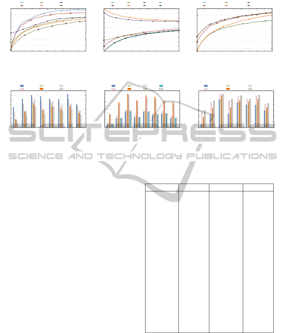
4 EMPIRICAL RESULTS

Figure 2 shows the reconstruction accuracy of the du-

plication and trigonometric interpolation approaches

for an increasing gap size. AWI and MWI achieved

a good interpolation for small gap sizes, but quickly

declined as the gap increased. LI struggled to re-

construct small gaps, but still outperformed AWI and

MWI for gaps of ﬁve samples and larger. CI had

the best accomplishment for gaps of two samples and

greater. The reconstruction performance of the algo-

rithms in ﬁgure 2 for different genres is given in ﬁgure

3. CI and AWI achieved the best and worst results re-

spectively for all genres. NNI and SI outperformed LI

in all genres, except classical music.

Figure 4 illustrates the interpolation NRMSE for

the examined polynomials over an increasing gap

size. The STP, SPS, NEP and HEP achieved almost

identical results. Since the best performing spline in-

terpolation utilizes linear piecewise polynomials, the

interpolation accuracy of the STP and SPS are equiv-

alent. The STP does not beneﬁt when employed in

an osculating fashion. However, the FOP improved

with the inclusion of derivatives and clearly beneﬁted

when applied as splines. An opposite trend is ob-

served for the FOP and OFP, where smaller gaps were

more difﬁcult to interpolate than larger gaps. This

trend is caused by a high frequency FOP ﬁtted over

smaller gaps. As the gap size increases, the frequency

of the sine and cosine waves decreases, providing a

smoother interpolation. Figure 5 shows the polynomi-

als’ interpolation performance for the different gen-

res. FOP and OFP had a clear inﬂation compared

to the other algorithms. OSP also had a slight surge,

with the rest of the algorithms achieving a similar in-

terpolation over all genres.

The time series models’ interpolation perfor-

mance for a growing duration is illustrated in ﬁgure

6. The AR and ARMA models had a similar per-

formance, whereas the ARIMA model started devi-

ating from the trend with gaps wider than eight sam-

ples. The ARCH and GARCH models had an iden-

tical trend, indicating that there is no difference be-

tween using and AR or ARMA process to predicting

SIGMAP2015-InternationalConferenceonSignalProcessingandMultimediaApplications

0.02

0.04

0.06

0.08

0.10

0.12

0.14

0.16

5 10 15 20 25 30 35 40 45 50

NRMSE

Gap Size (Samples)

AWI

MWI

NNI

Figure 2: The reconstruction of duplica-

tion methods for different gap sizes.

0.03

0.05

0.07

0.09

0.11

0.13

0.15

0.17

0.19

0.21

5 10 15 20 25 30 35 40 45 50

NRMSE

Gap Size (Samples)

STP

OSP

SPS

FOP

OFP

FPS

NEP

HEP

Figure 4: The reconstruction of polyno-

mials for different gap sizes.

0.02

0.04

0.06

0.08

0.10

0.12

0.14

5 10 15 20 25 30 35 40 45 50

NRMSE

Gap Size (Samples)

ARMA

ARIMA

ARCH

GARCH

Figure 6: The reconstruction of time se-

ries models for different gap sizes.

0.05

0.06

0.07

0.08

0.09

0.10

0.11

0.12

0.13

Classical

Country

Electro

Jazz

Metal

Pop

Reggae

Rock

NRMSE

Genre

AWI

MWI

NNI

Figure 3: The reconstruction of duplica-

tion methods for different genres.

0.05

0.06

0.07

0.08

0.09

0.10

0.11

0.12

0.13

0.14

0.15

Classical

Country

Electro

Jazz

Metal

Pop

Reggae

Rock

NRMSE

Genre

STP

OSP

SPS

FOP

OFP

FPS

NEP

HEP

Figure 5: The reconstruction of the

polynomials for different genres.

0.04

0.05

0.06

0.07

0.08

0.09

0.10

Classical

Country

Electro

Jazz

Metal

Pop

Reggae

Rock

NRMSE

Genre

ARMA

ARIMA

ARCH

GARCH

Figure 7: The reconstruction of the time

series models for different genres.

a music signal’s variance. On average a music sig-

nal’s variance is comparatively low compared to high

volatile ﬁnancial markets for which the ARCH and

GARCH models were originally intended and there-

fore do not perform as well as the AR and ARMA

models. The corresponding genre comparison for the

models in ﬁgure 6 is given in ﬁgure 7. The AR and

ARMA models performed best for all genres, fol-

lowed by the ARIMA, MA and then the ARCH and

GARCH models. Table 1 shows the overall recon-

struction accuracy, execution time and the tradeoff be-

tween the accuracy and computational time calculated

using equation (24). The ARMA model performed

the best on average, with just a minor improvement

over the AR model. All algorithms, except the OFP

and ARIMA model, can be executed in real time us-

ing a single thread. CI was on average the fastest. The

tradeoff in the last column shows that the AR model

achieved the most effective results for the given exe-

cution time. Although not a major improvement over

the ARMA model, the AR had a considerable lower

computation time, since it was estimated with a LLS

ﬁt and not an iterative gradient-based algorithm.

The reconstruction process was also perceptually

evaluated. The refurbished songs had a pleasant lis-

tening experience with little noise in the background,

mostly restricted to the song segments with a narrow

dynamic range, such as rests which are prominent in

classical music. Due to the subjective nature, differ-

ent hearing ranges and the participants’ difﬁculties to

distinguishing between the interpolation of some al-

Table 1: The average reconstruction accuracy, execution

time and tradeoff for the interpolation algorithms.

Algorithm NRMSE Time (s\s) SAT

AWI 0.111371 0.049794 1.098892

MWI 0.104806 0.051691 1.167703

NNI 0.090748 0.027313 1.348714

SI 0.087269 0.054413 1.402265

LI 0.093215 0.027908 1.313032

CI 0.081218 0.027128 1.506959

STP 0.080057 0.031490 1.528750

OSP 0.086014 0.034523 1.422878

SPS 0.080057 0.038588 1.528683

FOP 0.122412 0.068523 0.999724

OFP 0.117923 5.325502 1.015416

FPS 0.081493 0.033035 1.501807

NEP 0.080058 0.027329 1.528749

HEP 0.081066 0.027557 1.509767

AR 0.071764 0.092778 1.704671

MA 0.087952 0.029541 1.391575

ARMA 0.071709 2.435243 1.678909

ARIMA 0.080201 6.808781 1.464877

ARCH 0.089057 0.062245 1.374061

GARCH 0.089057 0.062378 1.374060

gorithms, the NRMSE was used as the principal mea-

surement of the reconstruction accuracy.

5 CONCLUSION

Twenty interpolation algorithms were analysed and

GramophoneNoiseReconstruction-AComparativeStudyofInterpolationAlgorithmsforNoiseReduction

benchmarked against each other in order to determine

their reconstruction ability on disrupted gramophone

recordings. Different approaches to interpolation

were considered, including duplication and trigono-

metric methods, polynomials and time series mod-

els. It was found that the ARMA model performed

the best with an average NRMSE of 0.0717. The CI

had the fastest execution time at 0.0271 s\s. The AR

model was the most effective approach by achieving

the best interpolation for a given time limit.

Future work includes the analyses of more com-

plex models, such as neural networks, that may in-

crease the interpolation accuracy. Further research

has to be done in other areas of audio processing, such

as VoIP, in order to determine how well the examined

algorithms perform with other types of noise and dif-

ferent audio sources, such as speech instead of music.

REFERENCES

Berndt, E. K., Hall, B. H., Hall, R. E., and Hausman, J. A.

(1974). Estimation and Inference in Nonlinear Struc-

tural Models. In Annals of Economic and Social Mea-

surement, volume 3, pages 653–665.

Bollerslev, T. (1986). Generalized Autoregressive Condi-

tional Heteroskedasticity. Journal of Econometrics,

31(3):307–327.

Box, G. E. P. and Jenkins, G. M. (1970). Time Series Anal-

ysis: Forecasting and Control. Holden-Day Series in

Time Series Analysis. San Francisco, CA.

Broyden, C. G. (1970). The Convergence of a Class of

Double-rank Minimization Algorithms. IMA Journal

of Applied Mathematics, 6(1):76–90.

Cho, J. (2007). Optimal Design in Regression and Spline

Smoothing. PhD thesis, Queen’s University, Canada.

CMU (2011). SoundScan may be under reporting US vinyl

sales. www.thecmuwebsite.com/article/soundscan-

may-be-under-reporting-us-vinyl-sales. 2015-04-16.

Ding, M., Bressler, S., Yang, W., and Liang, H. (2000).

Short-window Spectral Analysis of Cortical Event-

related Potentials by Adaptive Multivariate Autore-

gressive Modeling. Biological Cybernetics, 83:35–45.

Duchon, C. E. (1979). Lanczos Filtering in One and

Two Dimensions. Journal of Applied Meteorology,

18(8):1016–1022.

Engle, R. F. (1982). Autoregressive Conditional Het-

eroscedasticity with Estimates of the Variance of

United Kingdom Inﬂation. Econometrica, 50(4):987–

1007.

Fisher, R. A. (1935). The Design of Experiments. Oliver

and Boyd, Edinburgh, United Kingdom.

Gearhart, W. B. and Shultz, H. S. (1990). The Function sin

x/x. The College Mathematics Journal, 21(2):90–99.

Kastner, R., Hosangadi, A., and Fallah, F. (2010). Arith-

metic Optimization Techniques for Hardware and

Software Design. Cambridge, United Kingdom.

Newton, I. and Whiteside, D. T. (2008). The Mathematical

Papers of Isaac Newton, volume 1 of The Mathemati-

cal Papers of Sir Isaac Newton.

Nied

zwiecki, M. and Ciołek, M. (2014a). Elimination of

Impulsive Disturbances from Stereo Audio Record-

ings. In European Signal Processing Conference,

pages 66–70.

Nied

zwiecki, M. and Ciołek, M. (2014b). Localization of

Impulsive Disturbances in Archive Audio Signals us-

ing Predictive Matched Filtering. In IEEE Interna-

tional Conference on Acoustics, Speech and Signal

Processing, pages 2888–2892.

Nied

zwiecki, M., Ciołek, M., and Cisowski, K. (2015).

Elimination of Impulsive Disturbances From Stereo

Audio Recordings Using Vector Autoregressive

Modeling and Variable-order Kalman Filtering.

IEEE/ACM Transactions on Audio, Speech, and Lan-

guage Processing, 23(6):970–981.

Nied

zwiecki, M. and Cisowski, K. (2001). Smart Copy-

ing - A New Approach to Reconstruction of Audio

Signals. IEEE Transactions on Signal Processing,

49(10):2272–2282.

Richter, F. (2014). The LP is Back! www.statista.com

/chart/1465/vinyl-lp-sales-in-the-us. 2015-04-16.

Sidiroglou-Douskos, S., Misailovic, S., Hoffmann, H., and

Rinard, M. (2011). Managing Performance vs Accu-

racy Trade-offs with Loop Perforation. In ACM SIG-

SOFT Symposium, pages 124–134. ACM.

Slutzky, E. (1927). The Summation of Random Causes

as the Source of Cyclic Processes. Econometrica,

5(2):105–146.

Sprechmann, P., Bronstein, A. M., Morel, J.-M., and Sapiro,

G. (2013). Audio Restoration from Multiple Copies.

In International Conference on Acoustics, Speech and

Signal Processing, pages 878–882.

Stallmann, C. F. and Engelbrecht, A. P. (2015a). Digi-

tal Noise Detection in Gramophone Recordings. In

ACM International Conference on Multimedia, Bris-

bane, Australia. In review.

Stallmann, C. F. and Engelbrecht, A. P. (2015b). Gramo-

phone Noise Detection and Reconstruction Using

Time Delay Artiﬁcial Neural Networks. IEEE Trans-

actions on Systems, Man, and Cybernetics. In review.

Wals, J. L., Ahlberg, J., and Nilsson, E. N. (1962). Best

Approximation Properties of the Spline Fit. Journal

of Applied Mathematics and Mechanics, 11:225–234.

Whittle, P. (1951). Hypothesis Testing in Time Series Analy-

sis. PhD thesis, Uppsala University, Uppsala, Sweden.

Wile, R. R. (1990). Etching the Human Voice: The

Berliner Invention of the Gramophone. Association

for Recorded Sound Collections Journal, 21(1):2–22.

SIGMAP2015-InternationalConferenceonSignalProcessingandMultimediaApplications