Modeling of Nonlinear Dynamics of Active Components in Intelligent

Electric Power Systems

Konstantin Suslov

, Svetlana Solodusha

and Dmitry Gerasimov

Irkutsk State Technical Uuniversity, 83, Lermontov str., Irkutsk, Russia

Energy Systems Institute SB RAS, 130, Lermontov str., Irkutsk, Russia

Keywords: Smart Grid, Volterra Polynomials, Power Quality, Control Systems, Electric Power Systems.

Abstract: The research is aimed at developing algorithms for the construction of automated systems to control active

components of the electrical network. The construction of automated systems intended for the control of

electric power systems requires high-speed mathematical tools. The method applied in the research to describe

the object of control is based on the universal approach to the mathematical modelling of nonlinear dynamic

system of a black-box type represented by the Volterra polynomials of the N-th degree. This makes it possible

for the input and output characteristics of the object to obtain an adequate and fast mathematical description.

Results of the computational experiment demonstrate the applicability of the mathematical tool to the control

of active components of the intelligent power system.

1 INTRODUCTION

One of the main directions in power engineering is

the adoption of components applicable to the

implementation of a smart grid concept. This

requires:

• Transmission lines with variable characteristics

(active and reactive impedance components);

• Devices for electromagnetic conversion of energy

with wide capabilities to adjust parameters;

• Systems of energy storage and accumulation;

• Switching devices with a high breaking capacity

and large commutation life;

• Executive mechanisms that make it possible to act

on the active network components on-line by

changing the network parameters and topology.

An integral part of modern power system is

positioned sensors and current state variables in the

amount sufficient for the on-line estimation of the

network state in normal, emergency and post-

emergency conditions.

Therefore, the objective is to create control

systems which operate in real time and allow fast

generation of control signals to all active network

components in order to generate optimal control

actions.

This method of control is only possible if new

algorithms and techniques of power system control

are implemented, in particular when the methodology

on selection of input vectors that characterize

operating conditions of power systems in terms of

system topology are developed.

2 STATEMENT OF THE

PROBLEM

In order to estimate the objective current state it is

necessary to take into account the parameters

characterizing power quality.

The application of appropriate mathematical tools

will make it possible to solve the stated problem.

These mathematical tools should meet the

following requirements:

• appropriately reflect the object of control in the

entire range of change in its characteristics;

• afford the possibility of obtaining an adequate

mathematical description based on real

characteristics of the object;

• have high performance in its technical

implementation.

Generally speaking, the analysis of dynamic

characteristics of wind power unit is based on the

methods using differential equations. Most of the

researches are devoted to the specification of

characteristics of individual components of wind

turbine (Li, 2011, He, 2009), specification of various

195

Suslov K., Solodusha S. and Gerasimov D..

Modeling of Nonlinear Dynamics of Active Components in Intelligent Electric Power Systems.

DOI: 10.5220/0005411801950200

In Proceedings of the 4th International Conference on Smart Cities and Green ICT Systems (SMARTGREENS-2015), pages 195-200

ISBN: 978-989-758-105-2

 2015 SCITEPRESS (Science and Technology Publications, Lda.)

coefficients (Manyonge, 2012) or consideration of a

mechanical part of the turbine as a n-mass system

(Bhandari, 2014). In practice, the initial data are

known with some error. In this case, as a rule,

solutions to the inverse problem turn out to be

unstable with respect to an error in the initial data.

Therefore, to construct stable methods we use the

theory of ill-posed problems. (Kabanikhin, 2011).

It is also obvious that these mathematical tools are

difficult to use in the microprocessor software which

in turn makes it difficult to perform control.

The goal of this research is to test the algorithms

for the construction of computer-aided systems for

power system control, in which the mathematical

models are used in the form of integral Volterra

polynomials.

We will name only some of the research areas, in

which the Volterra integral power series find their

use. These are: modelling of technical systems

(Venikov and Sukhanov, 1982, Pupkov, 1976) and

electronic devices (Stegmayeer, 2004), nonlinear

identification of communications channels (Tong

Zhou and Giannakis, 1997, Cheng and Powers, 1998)

and visualization systems (Lin and Unbehauen,

1992), analysis of non-stationary time series (Minu

and Jessy, 2012), and description of automatic

feedback control systems (Belbas and Bulka, 2011).

Nowadays there are many methods for the

determination of dynamic characteristics, and the

universality of this mathematical apparatus makes it

possible to create the software for doing experiments

on computer. In particular, the Voltaire XL package

(American company Applied Wave Research) has

shown its performance in describing the electronic

scheme by the finite sums of the Volterra series.

An isolated electrical energy source represented

by a horizontal-axis wind turbine was used as a real

physical object (Solodusha, 2014).

3 REFERENCE DYNAMIC

SYSTEM

It should be noted that renewable energy sources are

an active component of modern electric power

systems. As a reference dynamic system, we will

consider a mathematical model of horizontal-axis

wind turbine represented using the techniques (Pronin

and Martyanov, 2012, Perdana, 2004, Sedaghat and

Mirhosseini, 2012)

in the following form:

1 0.035

()= ,

( ) 0.08 ( )

() 1

Zt bt

−



−





(1)

116 12.5

( ) = 0.22 0.4 ( ) 5 exp ,

() ()

Ct bt

zt zt



−+ −





(2)

()

()= ,

()

() ()

()=

2()

SC t V t

, (3)

() ()

tMt

dt J

−

(4)

where

(rad/s) is rotational speed of wind turbine

elements,

(N·m) is torque created by

aerodynamic force,

(N·m) is load resistance

torque,

(kg·m

) is moment of inertia of the wind

turbine rotating parts,

(kg·m

) is air density,

) is blade – swept area,

(m) is wind wheel

radius,

(deg) is blade lean angle,

(m/s) is wind

speed; dimensionless magnitudes:

C is wind

energy efficiency,

is speed, z is current value of

speed.

One of the key tasks is to reduce the dynamic

loads on the structure during strong winds. Control of

blade turning makes it possible to considerably

decrease the load on the structure. The research is

aimed at studying the impact of the blade lean angle

and wind speed

on the angular velocity of

rotation

4 INTEGRAL MODELS

The mathematical model of the input-output type

system can be represented by the Volterra polynomial

of the

N -th degree:

() ()

niip

yt f t

,...,

=≤≤...≤≤



(5)

()

1 n

,...,

()()

,, 1

ii n i m m

Kss xtsds

...

= ... ,..., −

∏



, (6)

where

[

]

0tT∈, ,

(1)

[0, ]

(0) 0, ( )

yytC=∈.

To construct an integral model in the form (5), (6)

means to restore multidimensional transient

characteristics of the nonlinear dynamic system

...

. Currently, there are quite many methods

developed to determine the dynamic characteristics

SMARTGREENS2015-4thInternationalConferenceonSmartCitiesandGreenICTSystems

196

(Doyle and Pearson, 2002, Rugh, 1981). The most

widely used approach is presented in (Danilov, 1990).

It suggests setting a multiparametric family of test

signals consisting of a combination of Dirac delta

functions to recover the Volterra kernels. However,

such an approach has limited application (Ljung,

1987).

The technique for the identification of (5), (6)

(Apartsyn, 2003, 2000, 2013) which is used in the

paper is based on setting a group of test signals

represented by special linear combinations of

Heaviside functions with deviating argument. Here

the problem of identification is reduced to solving the

Volterra linear integral equations of the first kind,

which allow explicit inversion formulas.

Further in (5), we will consider only the case

where

=2N

, which is the most important for

applications. The Volterra kernels will be identified

by the technique (Apartsyn, 2003, 2000, 2013), using

the midpoint rule to numerically solve (5), (6).

The numerical procedure for solving the system

(1) - (4) will be considered as a reference for the

assessment of the integral model accuracy. To

approximately solve (1) - (4) we apply the 4-th order

Runge-Kutta method.

The integral models are constructed to describe

the nonlinear dynamics of the output signal

() ()

TTT

ωωω

Δ= −in the case of scalar input

signal

()btΔ (or ()VtΔ ).

Below consideration is given to the case for the

input signal

()btΔ . Practical identification of

transient characteristics in the model

11111

() ( ) ( )

tKsbtsds=Δ−+



11 1 2 1 2 1 2

(, ) ( ) ( )

ss bt s bt sdsds+Δ−Δ−



(7)

was carried out on the basis of the experimental data

for the test disturbance signals

() (() ( )),b t et et

αω

Δ= −− () 0VtΔ=,

where

=± , 020t

≤≤≤ (s), ()et –

Heaviside function:

0, 0;

()

1, 0.





≥



Figure 1 presents the outputs of the reference

model (1)-(4) to the input disturbances

(, ) 10( () ( ))bt et et

ωω

Δ=−−−.

Figure 1: Experimental outputs.

(, )

The outputs

(, )

of the reference model (1)-

(4) took part in the recovery procedure of the sought

transient characteristics of the system in the scalar

model (7).

It should be specified that the recovery of kernels

()Kt,

(, )Ktt

− in (7) as a result of the

application of the approach (Apartsyn, 2003, 2000,

2013) can be reduced to solving special Volterra

linear integral equations of the first kind. Search for

the difference analog to the kernels

()Kt,

(, )Ktt

− was carried out on a uniform grid

tih= 1,in= , nh T= . The total number of the

unknowns taking part in the experiment of

constructing one model of form (7) was equal to

(1)

Along with the scalar model of form (7) we have

developed and implemented an algorithm for the

construction of the quadratic Volterra polynomial

2111

() ( ) ( )

yt Ksxt sds

=−+





12 1 2 12

(, )( )( )

ii i i

Kssxtsxtsdsds

+−−+





12121 1 2 2 12

(, )( ) ( )

Kssxtsxtsdsds+−−



(8)

For the case of vector input

() ( (), ())

txtxt= ,

where

() (),

tbt=Δ

() ()

tVt=Δ .

0 2 4 6 8 10 12 14 16 18 20

(t)

ModelingofNonlinearDynamicsofActiveComponentsinIntelligentElectricPowerSystems

197

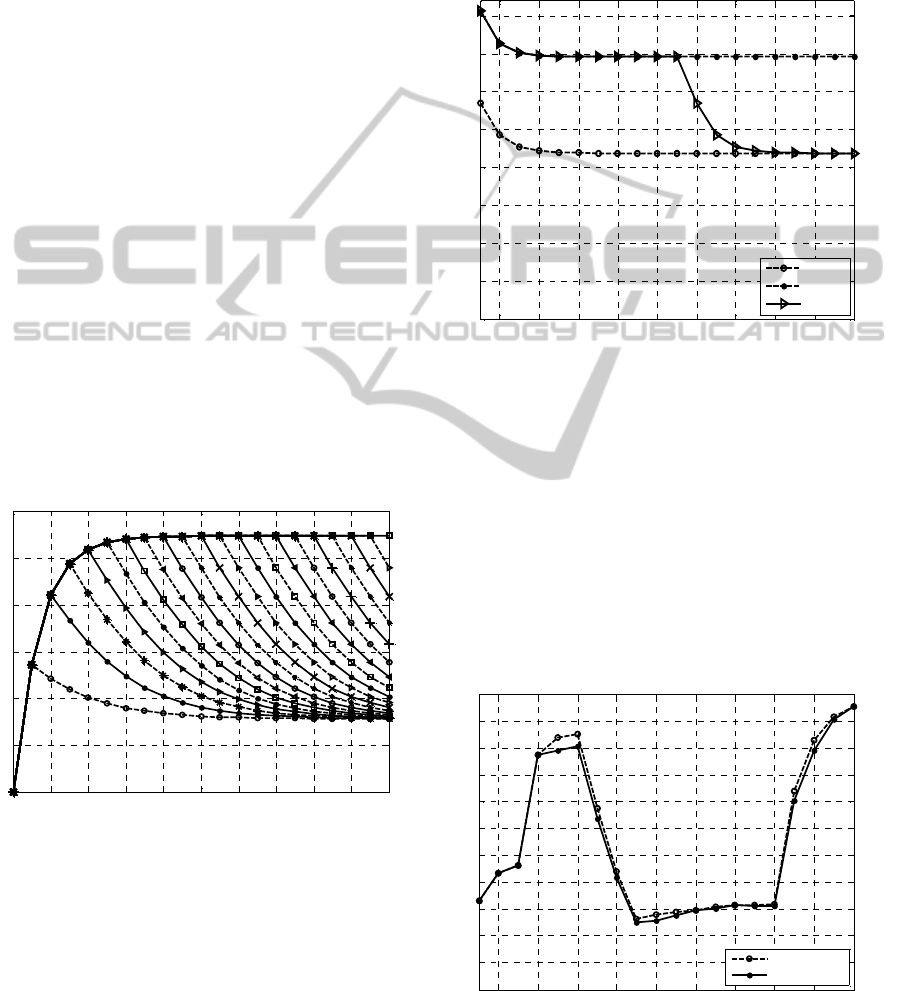
Figure 2 presents the output

(, )

of the

reference model (1)-(4) to the input disturbance of

form

(, ) 10( () ( )),

() 5(),

x t et et

xt et

ωω



=− − −









which was used in the recovery of the kernel

from the integral model (8).

The total number of the unknowns participating in

the experiment of constructing one model of form (8),

was equal to

2(1)nnn n+++.

5 CASE STUDY

The computational experiment consists of two stages.

In the first stage we build the integral models of form

(7), (8) by solving the problem of the identification of

transient characteristics of a dynamic system. In the

second stage we consider the problem of determining

the control action

() ()

tbt≡Δ , that maintains the

output signal

()

at a set level

. Considering

the transient characteristics

...

and output

()yt

in (7), (8) to be known, we determine the input signal

()

which corresponds to the specified output ()yt .

Figure 2: Experimental outputs.

(, )

In this section we present the results

demonstrating the first of the indicated stages of the

mathematical modeling. To ensure better accuracy,

the amplitude

of test signals used to determine the

Volterra kernels in (7), (8) was aligned with the

magnitude of the acting disturbances. It should be

noted that the model built using only one group of

signals cannot be considered equally suitable for the

calculation in the entire range of admissible changes

in the input signals. In order to improve the accuracy

of modeling we introduced reference initial

conditions for which the models of form (7) were

constructed. The calculations were performed on the

uniform grid with a step

=1h

(s).

Figure 3: Application of two integral models calculated

using (7). Notations: “model 1”, “model 2” are responses of

integral models for the reference integral model conditions

8V =

(m/s),

10V =

(m/s), respectively, “standard” –a

response of the standard model (1) - (4).

Figure 3 illustrates the application of the quadratic

Volterra polynomial (7) to forecast the output to the

input signals:

( ) 10( ( ) ( 11)) 8( ( 11)V t et et etΔ= −−+ −−

(20)),et−− () 10(),bt etΔ= [0,20]t ∈ ,

for

10b = (deg),

8V = (m/s),

10V = (m/s).

Figure 4: Comparison of the application of the integral

model of form (8) and the standard model (1)-(4).

0 2 4 6 8 10 12 14 16 18 20

(t)

2 4 6 8 10 12 14 16 18 20

(t)

model 1

model 2

standart

2 4 6 8 10 12 14 16 18 20

(t)

integral model

standart model

SMARTGREENS2015-4thInternationalConferenceonSmartCitiesandGreenICTSystems

198

Figure 4 illustrates the result of modeling the

output of the system

()

Δ to the input signals:

( ) 5( ( 3) ( 6)) 5( ( 6)V t et et etΔ= −−−− −−

( 16)),et−−

() 20(() ( 8))bt et etΔ = −−+

10( ( 8) ( 11)) 10( ( 16)et et et+−−−+−−

( 20))et−−

, [0,20]t ∈ ,

for

20b = (deg),

5V = (m/s) using the integral

model (8). The maximum relative error in

computations made up 4.4%.

Table 1 presents relative and absolute errors.

Table 1: Relative and absolute errors.

Examples of the

input signals

() 10(),bt etΔ=−

() 5()Vt etΔ=

0.00 0.000 0.00 0.00

() 20(),bt etΔ=−

() 10()Vt etΔ=

0.00 0.000 0.00 0.00

() 10(),bt etΔ=−

() 5(()Vt etΔ= −

(3))et−−

1.47 0.004 6.26 0.02

() 10( ()bt etΔ=− −

(1))et−−

() 5()Vt etΔ=

1.17 0.003 4.98 0.01

() 10(),bt etΔ=−

() 5(()Vt etΔ= −

( 12))et−−

1.89 0.068 8.04 0.29

() 20( ()bt etΔ=− −

(11))et−−

() 10()Vt etΔ=

1.39 0.102 5.91 0.43

() 20( ()bt etΔ=− −

(4))et−−

() 10()Vt etΔ=

1.28 0.006 5.45 0.03

() 20(),bt etΔ=−

( ) 10( ( )Vt etΔ= −

(1))et−−

1.29 0.007 5.49 0.03

The notations used in Table 1:

max | ( ) ( ) |

Ti i

tyt

εω

≤≤

=Δ −

(rad/s),

|()()|

TyT

εω

=Δ −

(rad/s),

100%

=⋅

(in %),

100%

=⋅

(in %),

20b = (deg),

5V = (m/s), ,

tih=⋅

1, 20i =

23.5

(rad/s), 1h = (s), 20T = (s).

The calculations show that the constructed

integral models describe the physical process with

admissible accuracy.

For solving (8) with respect to the control action

()

bt≡Δ

we use the algorithms developed in

(Solodusha, 2009). The study employs stable

difference methods in which a grid step is used as a

regularization parameter (Apartsyn, 2003). As

applied to the problem of automatic control it is

planned to compare the techniques for the

identification of Volterra polynomials of form (8)

which are based on the introduction of special classes

of piecewise constant test input signals. The analysis

of the studied approaches will allow us to identify the

preferable ranges for one or another algorithm, for the

reference model (1) - (4).

6 CONCLUSIONS

The presented results of the mathematical modeling

using the finite interval of the integro-power Volterra

series were for the first time applied to describe the

dynamics of the horizontal-axis wind turbine.

The technique was developed to construct the

integral model and technically implement the high-

speed system of control. A computational experiment

aimed at constructing the integral models of the wind

power unit was done.

The results of the computational experiment

demonstrates the applicability of this mathematical

tool to the control of active components of the electric

power system.

To improve the accuracy of modeling, it is

planned to introduce a structure with switchable

kernels, which will envisage the adaptive behavior of

the model in the case the input signal amplitudes go

beyond some limited interval.

The computer modeling was carried out using the

author’s software created in Matlab.

Further it is planned to apply this approach to the

research into complex dynamic systems which

contain an arbitrarily large amount of components of

the active-adaptive isolated system.

ACKNOWLEDGEMENTS

The research was partly funded by the grant of the

Russian Foundation of Basic Research, project

No.15-01-01425a.

ModelingofNonlinearDynamicsofActiveComponentsinIntelligentElectricPowerSystems

199

REFERENCES

He, Z., Xu Jianyuan, X., Xiaoyu, W., 2009. The dynamic

characteristics numerical simulation of the wind turbine

generators tower based on the turbulence model. In 4th

IEEE Conference on Industrial Electronics and

Applications. ICIEA 2009.

Li, J., Chen, J., Chen, X., 2011. Dynamic Characteristics

Analysis of the Offshore Wind Turbine Blades. Journal

Marine Sci. Vol.10, pp. 82-87.

Manyonge, A.W., Ochieng, R.M., Onyango, F.N.,

Shichikha, J.M., 2012. Mathematical Modelling of

Wind Turbine in a Wind Energy Conversion System:

Power Coefficient Analysis. Applied Mathematical

Sciences. Vol.6. No. 91, pp. 4527-4536.

Bhandari, B., Poudel, S.R., Lee, K.T., Ahn, S.Н., 2014.

Mathematical Modeling of Hybrid Renewable Energy

System: A Review on Small Hydro-Solar-Wind Power

Generation. International Journal of Precision

Engineering and Manufacturing-Green Technology.

Vol.1, No.2, pp.157-173.

Kabanikhin, S.I., 2011. Inverse and Ill-posed problems.

Theory and applications. Germany: De Gruyter,

Venikov, V.A., Sukhanov, O.A., 1982. Cybernetic models

of electric power systems. Moscow: Energoizdat, p.327

(in Russian).

Pupkov, K.A., Kapalin, V.I., Yushenko, A.S., 1976.

Functional Series in the Theory of Non-Linear Systems,

Moscow: Nauka. (in Russian).

Stegmayeer, G., 2004. Volterra series and neural networks

to model an electronic device nonlinear behaviour. In

IEEE International Conference on Neural Networks. V.

4, pp. 2907-2910.

Tong Zhou, G., Giannakis, G.B. 1997. Nonlinear channel

identification and performance analysis ,with PSK

inputs. In IEEE Signal Processing Workshop on Signal

Processing Advances in Wireless Communications, pp.

337-340.

Cheng, C.H., Powers, E.J., 1998. Fifth-order Volterra

kernel estimation for a nonlinear communication

channel with PSK and QAM inputs. In IEEE Signal

Processing Workshop on Statistical Signal and Array

Processing, pp. 435-438.

Lin, J.N., Unbehauen, R., 1992. 2-D adaptive Volterra filter

for 2-D nonlinear chanel equalization and image

restoration. Electronics Lett. No. 28(2). pp. 180-182.

Minu, K.K., Jessy, J. C., 2012. Volterra Kernel

Identification by Wavelet Networks and its

Applications to Nonlinear Nonstationary Time Series,

Journal of Information and Data Management. No. 1,

pp. 4-9.

Belbas, S.A., Bulka, Yu., 2011. Numerical solution of

multiple nonlinear Volterra integral equations. Applied

Mathematics and Computation, Vol. 217(9), pp. 4791-

4804.

Solodusha, S.V., Gerasimov, D.O., Suslov, K.V., 2014.

Modeling of Wind Turbine with Volterra Polynomials.

In VII International Symposium GSSCP

, pp. 161-163

(in Russian).

Pronin, N.V., Martyanov, À.S., 2012. Model of Wind

Turbine in the Package MATLAB. Bulletin of the South

Ural State University. Series Power Engeneering, No.

37(296), pp. 143-145 (in Russian).

Perdana, A., Carlson, O., Persson, J., 2004, Dynamic

Response of Grid-Connected Wind Turbine with

Doubly Fed Induction Generator during Disturbances.

In. IEEE Nordic Workshop on Power and Industrial

Electronics.

Sedaghat, A., Mirhosseini, M., 2012. Aerodynamic design

of a 300 kW horizontal axis wind turbine for province

of Semnan. Energy Conversion and Management. Vol.

63, pp. 87-94.

Doyle III, F., Pearson, R., Ogunnaike, B., 2002.

Identification and Control Using Volterra Models.

Springer-Verlag,

Rugh, W.J., 1981. Nonlinear System Theory: The

Volterra/Wiener Approach, Johns Hopkins University

Press, Baltimore, MD.

Danilov, L.V., Matkhanov, L.N., Filippov, V.S. 1990. A

Theory of Non-Linear Dynamic Circuits. Moscow:

Energoizdat (in Russian).

Ljung, L. System Identification. Theory for the User, 1987.

Apartsyn, A.S. Nonclassical linear Volterra equations of

the first kind. Boston: VSP Utrecht, 2003.

Apartsyn, A.S., Solodusha, S.V., 2000. Mathematical

simulation of nonlinear dynamic systems by Volterra

series. Engineering Simulation. Vol. 17, No. 2, pp. 143-

153.

Apartsyn, A.S., Solodusha, S.V., Spiryaev, V.A., 2013.

Modeling of Nonlinear Dynamic Systems with Volterra

Polynomials: Elements of Theory and Applications.

IJEOE, V. 2, No. 4, pp. 16-43.

Solodusha, S.V., 2009. A class of systems of bilinear

integral Volterra equations of the first kind of the

second order. Automation and Remote Control. Vol. 70,

No. 4, pp. 663-671.

SMARTGREENS2015-4thInternationalConferenceonSmartCitiesandGreenICTSystems

200