Finding Good Compiler Optimization Sets

A Case-based Reasoning Approach

Nilton Luiz Queiroz Junior and Anderson Faustino da Silva

Department of Informatics, State University of Maring´a, Maring´a, Brazil

Keywords:

Machine Learning, Metaheuristics, Cases-based Reasonig, Compiler Optimization Sets.

Abstract:

Case-Based Reasoning have been used for a long times to solve several problems. The ﬁrst Case-Based Rea-

soning used to ﬁnd good compiler optimization sets, for an unseen program, proposed several strategies to

tune the system. However, this work did not indicate the best parametrization. In addition, it evaluated the

proposed approach using only kernels. Our paper revisit this work, in order to present an detail analysis of an

Case-Based Reasoning system, applied in the context of compilers. In adition, we propose new strategies to

tune the system. Experiments indicate that Case-Based Reasoning is a good choice to ﬁnd compiler optimiza-

tion sets that outperform a well-engineered compiler optimization level. Our Case-Based Reasoning approach

achieves an average performance of 4.84% and 7.59% for cBench and SPEC CPU2006, respectively. In addi-

tion, experiments also indicate that Case-Based Reasoning outperforms the approach proposed by Purini and

Jain, namely Best10.

1 INTRODUCTION

Case-Based Reasoning (CBR) (Richter and Weber,

2013), an approach considered a subﬁeld of machine

learning (Mitchell, 1997; Shalev-Shwartz and Ben-

David, 2014), tries to solve a new problem using

a solution of an previous similar situation. It can

be seen as a learning process (Aamodt and Plaza,

1994), which stores past experiences in a knowledge

database, and can be updated incorporating new ex-

periences (Jimenez et al., 2011).

Over the years, this approach have been applied to

several problems, such as: estimate the project cost

to web hypermedia (Mendes and Watson, 2002), es-

timate the Q-factor of an optical network (Jimenez

et al., 2011), management of typhoon disasters (Zhou

and Wang, 2014), and estimate good compiler opti-

mization sets (Lima et al., 2013).

Compilers are programs that transform source

code from one language (source language) to an-

other (target language) (Aho et al., 2006; Srikant and

Shankar, 2007; Cooper and Torczon, 2011). During

this process, the compiler applies several optimiza-

tions (Muchnick, 1997), in order to improve the target

code. However, some optimizations can be good to a

class of programs, and bad to another. Then, the most

appropriate approach is to ﬁnd the best compiler op-

timizations to each program. The literature presents

different approaches to mitigate this problem (Zhou

and Lin, 2012; Lima et al., 2013; Purini and Jain,

2013). The ﬁrst CBR approach in this context (Lima

et al., 2013) indicates that it approach is able to in-

fer good solutions to new problems - good compiler

optimization sets to unseen programs.

In this paper we revisit the work of Lima et al.

(Lima et al., 2013) to explore new strategies of ﬁnding

good compiler optimization sets to a unseen program.

Lima et al. (Lima et al., 2013) used dynamic fea-

tures to representanalogies and a leave-one-outcross-

validation approach. Our work uses dynamic features

or static features to represent analogies. In addition,

our work uses different training and test datasets for

cross-validation.

The main contributions of this paper are:

• We describe different CBR parametrization.

• We give a new similarity metric to measure the

similarity between two programs.

• We present a program characterization approach

using static features.

• We present different strategies to build a collec-

tion of past experiences.

• We present a detail experimental analysis of CBR

approach in the context of compilers.

This paper is organized as follows. Section 2

presents related work. Section 3 explains brieﬂy

504

Queiroz Junior N. and da Silva A..

Finding Good Compiler Optimization Sets - A Case-based Reasoning Approach.

DOI: 10.5220/0005380605040515

In Proceedings of the 17th International Conference on Enterprise Information Systems (ICEIS-2015), pages 504-515

ISBN: 978-989-758-096-3

 2015 SCITEPRESS (Science and Technology Publications, Lda.)

CBR. Section 4 details our CBR approach, which goal

is to ﬁnd good compiler optimization sets. Section 5

presents the experimental setup. Section 6 details the

experimental results. Finally, Section 7 presents con-

clusions and future work.

2 RELATED WORKS

In the context of compilers, the work of Purini and

Jain ﬁnds a small set of compiler optimizations sets

(COS), which cover several programs (Purini and

Jain, 2013). Using iterative compilation, Zhou evalu-

ates a random and a genetic strategy, in order to ﬁnd

good compiler optimizations (Zhou and Lin, 2012).

Our work tries to mitigate the same problem. How-

ever, using a different approach.

Lima et al. proposed the ﬁrst CBR approach to

ﬁnd good COS to a unseen program. This approach

uses different strategies to select past results and mea-

sure the similarity between programs (Lima et al.,

2013). The work of Lima et al. does not indicate

which parametrization is the best. In addition, the

benchmark used is composed only by kernels. It is a

problem, in general we use complete applications and

not kernels. Therefore, we revisit this work in order

to cover these gaps.

Jimenez used a CBR approach to estimate Q-

factor in optical networks. His approach obtained

a successful classiﬁcation in 94% of cases (Jimenez

et al., 2011). Erbacher used a same approach to auto-

matically report hostile actors in a network (Erbacher

and Hutchinson, 2012). To implement a system able

to generate combat strategies, Kim et al. (Kim et al.,

2014) proposed a CBR approach that retrieves past

experiences and modify them to the current situation.

The main difference between these works and the our

is the context where the CBR is applied.

3 CASE-BASED REASONING

CBR, a machine learningapproach, can be subdivided

in four processes:

1. Retrieve a case from a collection of (past experi-

ences) previous cases by similarity measure.

2. Reuse the knowledge of an old case to solve a new

case.

3. Revise the result of this new case, evaluating the

success of the solution.

4. Retain the useful experience for future reuses.

Every CBR, in specially the retrieve process,

needs some parameters, such as:

Collection guide indicates the strategy used to build

the collection of previous cases.

Similarity measure measures the level of similarity

between a previous case and a new one.

Standardization transforms all attributes values ac-

cording to a speciﬁc rule.

Number of analogies indicates the number of previ-

ous cases that will be used to estimate a solution

to an unseen problem.

In general, the cases that compose the collection

of previous cases come from real world experiences.

However, in our context, there is not a public real

world collection, used by the scientiﬁc community.

Therefore, we need to generate a collection of past

experiences to use it as previous cases.

4 FINDING GOOD COMPILER

OPTIMIZATION SETS USING A

CBR APPROACH

The main goal of the CBR described in this paper

is to ﬁnd a COS, which is able to achieve a perfor-

mance improvement over a well-engineered compiler

optimization level.

The CBR approach divides the process of ﬁnding

an effective COS into:

1. An ofﬂine phase; and

2. An online phase.

The ofﬂine phase collects pieces of information

about a set of training programs, and downsamples

the search space in order to provide a small space,

which can be handled by the online phase in a easy

and fast way. Therefore, the ofﬂine phase creates a

collection of previous cases, which will be used to

determine the knowledge that will be used to solve an

unseen case, in other words, to determine a COS that

should be enabled on an unseen program.

The online phase will infer from the cases pro-

vided by the ofﬂine phase, the best COS that ﬁts the

feature of unseen program as deﬁned by its input.

4.1 The Ofﬂine Phase

The ofﬂine phase builds a collection of previous cases

storing for training programs several success cases.

It means that the downsampling technique should

be guided to retain good cases, besides pruning the

FindingGoodCompilerOptimizationSets-ACase-basedReasoningApproach

505

Algorithm 1: Ofﬂine Phase.

Input: Ps // Training programs

B // Baseline

Output: A collection of cases

collection ← [ ]

for each P ∈ Ps do

sets ← [ ]

info ← { };

// Compile the program P using

// the highest compiler level (baseline),

// and get the number of

// hardware instructions executed

bas ← getPerformance(B, P)

while not reach the stop condition do

// Generate a new and unique case, i. e.,

// a compiler optimization set

case ← generateCase()

// Compile the program P using the

// new case, and get the number

// of hardware instructions executed

value ← getPerformance(case, P)

sets.append((case, value))

// Get the feature of program P,

// and normalize it

inf o ← getNormalizedFeature(P)

collection.append((P.name, info, bas, sets))

return collection

search space. The Algorithm 1 describes brieﬂy the

ofﬂine phase.

Algorithm 1 indicates that the feature for each

training program is normalized. It is performed by the

ofﬂine phase, due to different programs have different

features, for example the number of hardware instruc-

tions executed, runtime, and others. In addition, each

feature should be collected compiling and running the

training program without any compiler optimization

enabled. It guarantees that the optimizations will not

inﬂuence the program behavior.

4.2 The Online Phase

The online phase performs the CBR, in order to ﬁnd

an effective COS, which should be enabled on the

unseen (test) program. The Algorithm 2 describes

brieﬂy this phase.

For the test program, the online phase collects its

features and compares them with the features of each

training program, with the help of a similarity model

that ranks the training programs. This rank indicates

what training program is the most similar to test pro-

gram. In summary, the online phase selects from the

most similar training programs previous cases, evalu-

ates these cases and returns the best one.

Algorithm 2: Online Phase.

Input: C // Collection

P // Test program

B // Baseline

N // Number of analogies (cases)

S // Similarity

Output: The best case

cases ← [ ]

best

case ← B

// Compile the program P using the baseline,

// and get the number of hardware

// instructions executed

best

per f ← getPerformance(B, P)

// Get the features of the program P,

// and normalize them

inf o ← getNormalizedInformation(P)

// Build a collection with only success cases

// (cases that improved the performance

// of training programs)

′

← filterCollection(C)

// Rank the training programs

// based on similarity model S

rank ← getRank(C

′

, info, S)

// Get the potential previous cases

cases ← getAnalogies(C

′

, L,rank)

// Evaluate the potential cases

for each case ∈ cases do

// Compile the program P using the

// case, and get the number

// of hardware instructions executed

per f ← getPerformance(case, P)

if per f < best

per f then

best per f ← perf

best case ← case

return best case, best perf

4.3 Parametrization

The parametrization of our CBR is as follows.

Collection Guide. Several strategies can be used to

build a collection of previous cases. In our work,

we use iterative and metaheuristic algorithms to

perform this task. The iterative algorithm gener-

ates the collection by a uniform random sampling

of the optimization space. While, the metaheuris-

tic algorithms use a sophisticated way to build a

collection. The metaheuristic are genetic algo-

rithm with rank selection, genetic algorithm with

tournament selector, and simulated annealing. In

addition, we build a collection that is composed

by all the previous collections.

ICEIS2015-17thInternationalConferenceonEnterpriseInformationSystems

506

Similarity Model. In order to measure the similarity

between two programs, the CBR system can be

tunned to use a strategy chosen from:

Cosine. In this model, the similarity between P

and P

is deﬁned as:

sim(F

, F

) =

∑

w=1

×F

∑

w=1

)

∑

w=1

)

Jaccard. In this model, the similarity between F

and F

is deﬁned as:

sim(F

, F

) =

∑

w=1

min(F

)

max(F

)

Euclidean. In this model, the similarity between

and F

is deﬁned as:

sim(F

, F

) =

√

∑

w=1

−F

)

In both models, m is the quantity of features. The

ﬁrst two similarity models were proposedby Lima

et al. (Lima et al., 2013). In our work, we use

these two models and a model based on Euclidean

distance. As mentioned previously by Lima et al.,

these models are based on similarity coefﬁcients

used to compare statistical sampling, and indicate

that large difference between two feature vectors

should return a low similarity value.

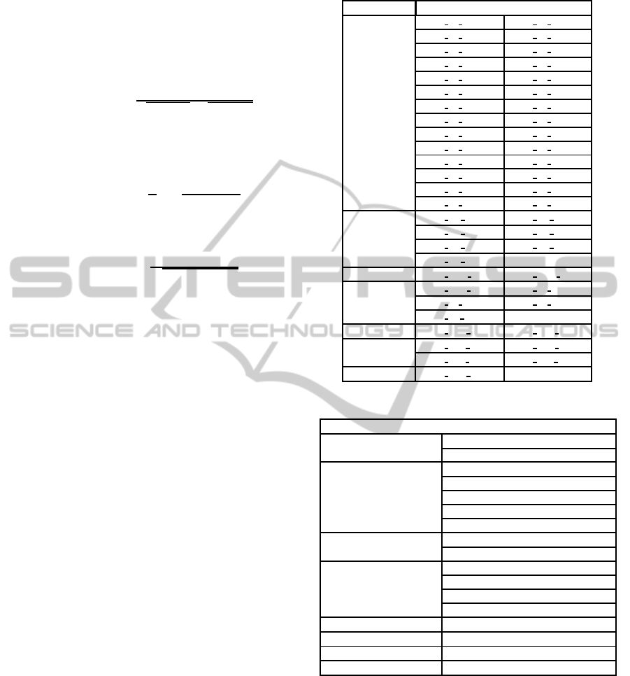
Feature. A similarity model measures the similarity

between two programs, based on their features.

Our CBR is able to use dynamic or static fea-

tures to describe the program behavior. Dynamic

features are composed by hardware performance

counters (Mucci et al., 1999), which describe the

program behavior during its execution. Static fea-

tures are composed by compiler statistics, which

describe the program behavior during its compila-

tion. Table 1 presents the dynamic features used

in our work, and Table 2 presents the static fea-

tures. In addition, these tables indicate the most

important feature (*). Our CBR system can use

all features, only the most important features, or

a weighted strategy. In the weighted strategy the

feature vectors are weighted to reﬂect the relative

importance of each feature. In our system, the

weight of an important feature has value 2, while

the other has value 1.

Standardization. The system should divide each

feature for the most important one (**). It trans-

forms all attributes values in order to standardize

the features of training and test programs.

Number of Analogies. The best strategy is to choose

several analogies to increase the probability of

Table 1: Dynamic Feature.

Type Performance Counter

Cache

PAPI L2 DCR PAPI L3 DCR

PAPI L2 TCA

∗

PAPI L3 TCA

PAPI L2 DCW PAPI L3 DCW

PAPI L1 ICM PAPI L2 STM

PAPI L1 DCM PAPI L3 TCM

PAPI L2 TCM PAPI L3 TCR

PAPI L2 TCR PAPI L3 DCA

PAPI L2 DCA PAPI L3 TCW

PAPI L2 TCW PAPI L2 ICR

PAPI L2 DCH

∗

PAPI L1 STM

PAPI L1 TCM PAPI L1 LDM

PAPI L2 DCM PAPI L2 ICA

PAPI L3 ICR PAPI L2 ICM

PAPI L3 ICA PAPI L2 ICH

∗

Branch

PAPI BR PRC PAPI BR UCN

PAPI BR NTK PAPI BR INS

∗

PAPI BR MSP PAPI BR TKN

PAPI BR CN

SIMD PAPI VEC SP

∗

PAPI VEC DP

∗

Floating Point

PAPI FDV INS PAPI FP INS

PAPI FP OPS PAPI SP OPS

PAPI DP OPS

TLB PAPI TLB DM

∗

PAPI TLB IM

Cycles

PAPI REF CYC PAPI TOT CYC

∗

PAPI STL ICY PAPI STL ICY

Instructions PAPI TOT INS

∗∗

Table 2: Static Feature.

Static Data

Binary Instructions

Number of Add insts

Number of Sub insts

Memory Instructions

Number of Store insts

∗

Number of Load insts

∗

Number of memory instructions

∗

Number of GetElementPtr insts

Number of Alloca insts

Terminator Instructions

Number of Ret insts

Number of Br insts

Other Instructions

Number of ICmp insts

Number of PHI insts

Number of machine instrs printed

∗

Number of Call insts

Function Number of non-external functions

Basic block Number of basic blocks

Floating Point Instructions Number of ﬂoating point instructions

∗

Total Instructions Number of instructions (of all types)

∗ ∗∗

choosing a good one. Our system is able to eval-

uate several number of cases. However, the most

similar training program can not be able to pro-

vide the required number of analogies. If it is the

case, the second most similar program will pro-

vide it, and so on.

FindingGoodCompilerOptimizationSets-ACase-basedReasoningApproach

507

5 EXPERIMENTAL SETUP

In our experiments, we will evaluate different conﬁg-

urations of our CBR system. The main conﬁguration

of the experimental environment is given by:

Hardware. We used a machinewith a Intel processor

Core I7-3779, 8 MB of cache, and 8 GB of RAM.

Operating System. The operating system was

Ubuntu 14.04, with kernel 3.13.0-37-generic.

Compiler. We adopted LLVM 3.5 (Lattner and

Adve, 2004; LLVM Team, 2014) as compiler in-

frastructure.

Baseline. The baseline is the LLVM’s highest com-

piler optimization level, -O3. The baseline indi-

cates the threshold that our system should over-

come.

Optimizations. The optimizations used to compose

a case are present in Table 3. We use only the

optimizations used by the highest compiler opti-

mization level -O3.

Table 3: LLVM’s optimizations used by -O3.

Optimizations

-inline -prune-eh -scalar-evolution

-argpromotion -inline-cost -indvars

-gvn -functionattrs -loop-idiom

-slp-vectorizer -sroa -loop-deletion

-globaldce -domtree -loop-unroll

-constmerge -early-cse -memdep

-targetlibinfo -lazy-value-info -memcpyopt

-no-aa -jump-threading -sccp

-tbaa -loop-unswitch -dse

-basicaa -tailcallelim -adce

-notti -reassociate -barrier

-globalopt -loops -branch-prob

-ipsccp -loop-simplify -block-freq

-deadargelim -lcssa -loop-vectorize

-instcombine -loop-rotate -strip-dead-prototypes

-simplifycfg -licm -verify

-basiccg -correlated-propagation

Cases. The process of creating a case is guided by

the criteria:

• Every optimization appears only once in a case;

• Every optimization can appear in any position;

• Every optimization should address the compi-

lation infrastructure rules; and

• All cases have the same length.

The ﬁrst criterion indicates that the ofﬂine phase

does not explore the use of one optimization sev-

eral times. Although, this occurs in LLVM’s -O3

optimization level. Second can be viewed as an

organization of the case (or COS). In the collec-

tion, every case is represented as a sequenceof op-

timizations. It means that there is a predeﬁned or-

der to apply each speciﬁc optimization. The third

indicates that a new case can not violate the safety

of the infrastructure. By the fourth criterion, the

ofﬂine phase tries to give to every case the same

characteristic.

Collection Guide. The creation of the collections

was guided as follows.

Random. This iterative algorithm generates in a

random way 500 cases.

Genetic Algorithm with Rank Selector. The

parameters chosen in this strategy were:

chromosome

size ← 40 (the number of op-

timizations in a case), population ← 60,

generation ← 100, mutation

rate ← 0.02,

and crossover rate ← 0.9. The algorithm will

ﬁnish whether the standard deviation of the

current ﬁtness score is less than 0.01 or the

best ﬁtness score does not change in three

consecutive generations. In addition, this

strategy uses elitism. It means that the best

solution of the generation N − 1 is kept in

generation N.

Genetic Algorithm with Tournament Selector.

It is similar to the previous strategy, but instead

of using a rank selector it uses a tournament

selector.

Simulated Annealing. In this strategy, the ini-

tial temperature is the half of hardware instruc-

tions executed, the perturbation function only

changes one random optimization in a random

position, the acceptance probability is given by

the Equation 1, and the temperature is adjusting

multiplying it by the constant α, which value is

0.95. The stop criteria is 500 iterations.

P(N) = e

−

∆(C)−∆(N)

(1)

All. This strategy only merges the previous col-

lections.

Training Programs. For the generation of the col-

lections of previous cases, we used 61 microker-

nel programs take from LLVM’s test-suite. All

the programs are single-ﬁle, and have short run-

ning times. Table 4 shows the microkernels.

Test Programs. We used for evaluating our CBR ap-

proach the benchmarks, cBench (cBench, 2014)

with dataset 1, and SPEC CPU2006 (Henning,

2006) with training dataset.

Validation. The results is based on the arithmetic

average of ﬁve executions, excluding the best

ICEIS2015-17thInternationalConferenceonEnterpriseInformationSystems

508

Table 4: Microkernels.

Microkernel programs

ackermann hash perlin

ary3 heapsort perm

bubblesort himenobmtxpa pi

chomp huffbench puzzle

dry intmm puzzle-stanford

dt lists queens

fannkuch lowercase queens-mcgill

fbench lpbench quicksort

ffbench mandel-2 random

ﬁb2 mandel realmm

ﬂdry matrix recursive

ﬂops-1 methcall reedsolomon

ﬂops-2 misr richards benchmark

ﬂops-3 n-body salsa20

ﬂops-4 nestedloop sieve

ﬂops-5 nsieve-bits spectral-norm

ﬂops-6 objinst strcat

ﬂops-7 oourafft towers

ﬂops-8 oscar treesort

ﬂops partialsums whetstone

fp-convert

and the worst values. In the experiments, the

machine workload was minimum as possible, in

other words, each instance was executed sequen-

tial. In addition, the machine did not have exter-

nal interference,and the runtime variance was less

than 0.01.

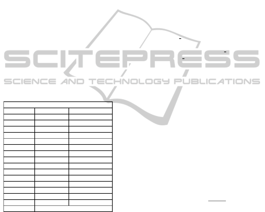
5.1 An Overview of the Collections

To analyze the improvement obtained by each strat-

egy of creating the collections, we summaries the col-

lections in Table 5. In this table, the column #P means

the number of programs with good cases.

Table 5: Summary.

Good Worst Best

Collection #P #Sets

Cases (%) Perf. (%) Perf. (%)

Random 55 30500 19.57 -99.99 58.33

Genetic

Algorithm 57 27973 39.42 -99.99 51.87

Rank

Genetic

Algorithm 56 27543 56.77 -99.99 51.87

Tournament

Simulated

Annealing

45 30500 7.42 -99.99 54.22

All 57 116455 30,54 -99.99 58.33

Most cases generated by simulated annealing do

not overcome the baseline. However, this strategy

was able to ﬁnd some cases that achieve a good im-

provement over the baseline. It indicate this strategy

has difﬁculty to escape from some bad improvement,

which is probably due to the disturbing function (the

function that chooses the neighbor). Besides, the ini-

tial solution inﬂuences the ﬁnal result, which could be

the source to several cases achieve bad improvements.

The overview of the other strategies shows a dif-

ferent scenario. The genetic algorithms generated a

better distribution. They have more success cases, if

we take the average as criteria to evaluate the col-

lection quality. However, if we take the maximum

improvement obtained for each program, simulated

annealing generates better results than genetic algo-

rithms, and random strategy.

These differences can be justiﬁed by the charac-

teristics of each implementation. Simulated anneal-

ing just change one optimization in each new case,

while the others metaheuristics try more changes in

each new case.

The number of cases is a small portion of the opti-

mization space. It indicates that the strategies used to

generate the collections was able to downsample the

search space in order to provide a small space with

good cases.

6 EXPERIMENTAL RESULTS

The goal of our CBR approach is to ﬁnd a COS that

outperforms the well-engineered compiler optimiza-

tion level -O3, in terms of hardware instructions exe-

cuted.

Our experiments was conducted in a way to an-

swer the following questions:

• What is the best parametrization of the CBR ap-

proach applied in the context of compilers?

• What is the best characterization of programs?

• What is the improvementobtained by the CBR ap-

proach in real applications?

• What is the best strategy to create a collection of

previous cases?

Tables 6 and 7 show the results obtained by each

CBR conﬁguration. In these tables, API stands for

average percentage improvement, APIE stands for

average percentage improvement excluding the pro-

grams showing no improvement, and NPI stands for

the number of programs achieving improvement.

Strategies that use static features do not generate

different results. It means that the use of these con-

ﬁgurations always ranks the training programs in the

same way. It explains the use of only one entry for

static features.

6.1 Overview

Collection Guide. Analyzing the different strategies

to construct the collections shows that the random

FindingGoodCompilerOptimizationSets-ACase-basedReasoningApproach

509

Table 6: Results obtained by cBench.

cBench 1 Analogy 3 Analogies 5 Analogies

Base Similarity API APIE NPI API APIE NPI API APIE NPI

Genetic

Algorithm

Rank

Selection

(GR)

Dynamic

Feature

(DF)

All

(AL)

Cosine -1.88 5.91 12 -1.12 6.58 14 0.71 7.15 19

Jaccard -2.86 5.55 13 -1.61 5.78 16 -1.21 5.8 17

Euclidean -1.18 6.27 13 -0.62 6.45 15 0.7 6.7 19

Most

Informative

(MI)

Cosine -5.51 3.58 13 -3.41 4.28 14 -1.47 6.32 16

Jaccard -1.89 4.81 13 -0.56 5.28 17 0.18 5.79 18

Euclidean -0.4 4.57 14 0.09 4.83 16 1.5 5.35 20

Weight

(WE)

Cosine -2.13 5.94 12 -1.02 6.49 14 0.79 7.07 19

Jaccard -2.86 5.55 13 -1.61 5.78 16 -1.03 6.11 17

Euclidean -1.02 6.29 13 -0.46 6.07 16 0.78 6.39 20

Static

Feature

(SF)

Cosine -7.59 5.45 8 -6.8 5.15 10 -6.71 5.15 10

Jaccard -1.88 5.84 16 0.17 5.77 18 0.19 5.79 18

Euclidean -4.28 6.06 12 -3.71 6.03 13 -3.41 5.61 14

Genetic

Algorithm

Tournament

Selection

(GT)

Dynamic

Feature

(DF)

All

(AL)

Cosine -1.87 4.4 15 -0.41 4.97 18 0.1 5.52 18

Jaccard -1.52 4.97 16 0.14 5.83 18 0.48 5.95 19

Euclidean -1.87 4.4 15 -0.41 4.97 18 0.1 5.52 18

Most

Informative

(MI)

Cosine -4.38 4.31 13 -2.69 5.87 14 -2.28 6.06 15

Jaccard -3.77 4.39 13 -1.23 6.13 17 -0.82 5.92 19

Euclidean -2.8 3.5 15 -1.5 3.67 18 -1.06 4.08 18

Weight

(WE)

Cosine -1.61 4.03 16 -0.45 4.45 19 0.05 4.92 19

Jaccard -1.85 4.97 16 -0.19 5.83 18 0.15 5.95 19

Euclidean -0.57 4.12 15 0.61 4.54 18 1.26 4.98 19

Static

Feature

(SF)

Cosine -5.84 4.02 11 -5.54 4.16 12 -5.43 4.17 12

Jaccard -2.66 6.02 13 -2.21 5.63 16 -1.82 5.63 16

Euclidean -3.31 3.67 13 -2.16 5.11 14 -2.11 5.13 14

Simulated

Annealing

(SA)

Dynamic

Feature

(DF)

All

(AL)

Cosine -4.97 3.88 12 -2.04 5.78 17 -1.72 5.87 18

Jaccard -2.97 6.29 16 0.79 7.11 18 2.35 6.64 20

Euclidean -5.89 4.39 10 -3.43 6.94 13 -2.8 6.58 16

Most

Informative

(MI)

Cosine -8.73 4.94 8 -1.65 6.25 13 0.74 6.39 17

Jaccard -4.19 5.46 13 -0.4 6.38 18 0.32 6.37 19

Euclidean -6.12 1.69 11 -3.57 3.85 17 -2.02 6.2 18

Weight

(WE)

Cosine -5.68 4.13 11 -2.75 6.07 16 -2.42 6.46 16

Jaccard -3.1 6.69 15 0.52 7.27 17 1.87 6.93 18

Euclidean -6.36 4.39 10 -3.83 6.6 14 -3.31 6.94 15

Static

Feature

(SF)

Cosine -8.88 4.73 9 -1.49 5.56 15 -0.93 5.37 18

Jaccard -4.4 3.66 9 -2.01 4.08 17 -1.25 4.72 18

Euclidean -5.25 4.54 12 -0.86 6.04 15 0.04 5.92 19

Random

(RA)

Dynamic

Feature

(DF)

All

(AL)

Cosine -3.16 5.23 11 1.21 6.28 20 1.92 6.88 21

Jaccard -3.25 7.11 10 0.05 6.62 16 1.14 6.59 19

Euclidean -2.95 4.84 12 1.05 6.03 20 1.82 6.73 21

Most

Informative

(MI)

Cosine -2.01 5.41 11 1.04 6.43 18 2.14 6.39 22

Jaccard -0.98 6.6 13 2.02 6.52 19 2.58 6.84 20

Euclidean -3.06 3.24 12 2.02 5.18 22 3.05 6.24 23

Weight

(WE)

Cosine -2.49 5.23 11 1.14 6.18 20 1.83 6.78 21

Jaccard -3.42 6.9 10 -0.04 6.35 16 1.05 6.37 19

Euclidean -1.72 5.12 12 2.2 6.41 19 2.92 7.02 20

Static

Feature

(SF)

Cosine -3.34 6.71 11 0.5 6.47 18 1.46 7.27 19

Jaccard 0.27 7.78 15 3.0 7.28 20 3.95 7.61 22

Euclidean -5.81 4.98 13 0.21 5.39 21 1.28 6.44 21

All

(AL)

Dynamic

Feature

(DF)

All

(AL)

Cosine 0.45 3.86 16 2.43 5.52 20 3.16 5.97 20

Jaccard -3.53 5.35 16 0.38 5.65 20 0.61 5.65 20

Euclidean 0.56 3.8 15 2.67 5.06 20 3.17 5.27 21

Most

Informative

(MI)

Cosine -7.38 2.53 8 -2.17 7.36 12 -1.12 7.31 15

Jaccard -4.69 4.99 11 -0.77 5.79 19 -0.67 5.9 19

Euclidean -3.88 3.95 9 -1.24 5.43 15 1.29 4.75 21

Weight

(WE)

Cosine -1.46 4.1 15 0.6 5.36 19 1.36 5.59 20

Jaccard -3.53 5.35 16 0.38 5.65 20 0.61 5.65 20

Euclidean 0.65 3.81 15 2.78 5.07 20 3.33 4.86 23

Static

Feature

(SF)

Cosine -6.82 3.01 10 -5.36 3.66 12 -5.06 3.89 13

Jaccard -3.21 3.61 12 -1.24 5.12 18 -1.03 4.86 19

Euclidean -6.96 3.37 10 -1.83 5.12 14 -1.54 5.22 15

ICEIS2015-17thInternationalConferenceonEnterpriseInformationSystems

510

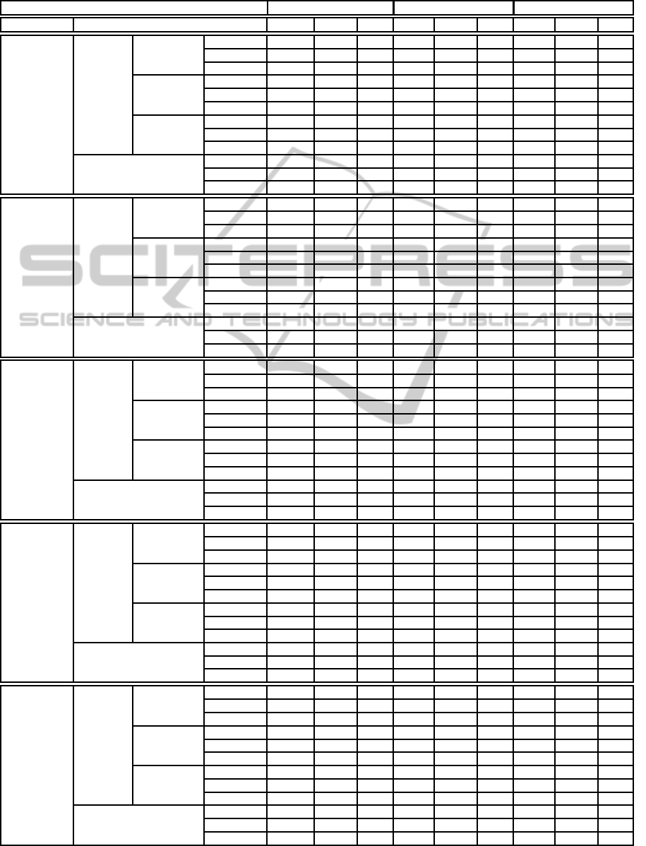
Table 7: Results obtained by SPEC CPU2006.

SPEC CPU2006 1 Analogy 3 Analogies 5 Analogies

Base Similarity API APIE NPI API APIE NPI API APIE NPI

Genetic

Algorithm

Rank

Selection

(GR)

Dynamic

Feature

(DF)

All

(AL)

Cosine -3.56 6.61 7 -2.46 7.09 7 -1.88 6.73 8

Jaccard -6.4 5.06 6 -4.96 7.56 6 -4.33 6.92 7

Euclidean -3.12 5.48 8 -1.9 6.14 8 -1.29 6.07 9

Most

Informative

(MI)

Cosine -5.55 6.62 7 -1.34 7.15 8 -0.63 6.96 9

Jaccard -8.67 5.81 6 -4.8 5.55 8 -0.41 5.09 9

Euclidean -6.35 5.34 7 -5.15 5.1 8 -4.25 5.03 9

Weight

(WE)

Cosine -3.93 7.18 6 -2.82 7.74 6 -2.24 7.24 7

Jaccard -6.4 5.06 6 -4.96 7.56 6 -4.33 6.92 7

Euclidean -3.42 5.44 8 -2.21 6.1 8 -1.6 6.04 9

Static

Feature

(SF)

Cosine -12.03 2.97 2 -8.39 2.42 3 -7.97 2.97 4

Jaccard -5.58 5.09 4 -4.92 5.15 4 -4.58 4.32 5

Euclidean -11.71 2.58 3 -8.08 2.27 4 -7.81 3.18 4

Genetic

Algorithm

Tournament

Selection

(GT)

Dynamic

Feature

(DF)

All

(AL)

Cosine -3.4 4.86 7 -2.9 5.4 7 -2.74 5.79 7

Jaccard -1.63 5.99 7 -1.11 6.11 8 -0.56 6.61 8

Euclidean -4.57 4.86 7 -4.12 5.4 7 -3.96 5.79 7

Most

Informative

(MI)

Cosine -8.34 4.42 5 -4.91 4.25 7 -2.87 4.64 7

Jaccard -7.09 7.45 5 -5.71 6.24 7 -2.89 6.9 7

Euclidean -5.15 4.49 8 -1.21 6.99 9 -0.82 6.9 10

Weight

(WE)

Cosine -4.87 4.68 8 -1.81 5.32 9 -1.65 5.63 9

Jaccard -2.35 5.99 7 -1.84 6.11 8 -1.3 6.61 8

Euclidean -5.31 5.07 8 -2.37 5.4 9 -2.21 5.72 9

Static

Feature

(SF)

Cosine -8.65 3.45 6 -8.12 3.25 7 -7.71 3.25 7

Jaccard -3.26 3.14 7 -2.72 3.14 8 -2.26 3.16 8

Euclidean -8.6 3.5 6 -8.09 3.3 7 -7.68 3.3 7

Simulated

Annealing

(SA)

Dynamic

Feature

(DF)

All

(AL)

Cosine -3.12 9.07 3 -1.32 8.37 6 -1.05 7.18 7

Jaccard -8.13 6.12 7 -1.91 7.89 7 -1.59 8.07 7

Euclidean -3.12 9.07 3 -1.28 7.26 7 -0.94 6.53 8

Most

Informative

(MI)

Cosine -3.93 8.1 6 -2.3 9.35 7 -1.63 9.7 7

Jaccard -4.97 5.55 7 -1.26 7.45 8 -0.07 7.57 8

Euclidean -6.15 11.38 2 -3.47 8.87 5 -2.65 8.78 6

Weight

(WE)

Cosine -3.4 9.07 3 -1.67 9.04 5 -1.16 6.87 7

Jaccard -8.65 4.7 7 -2.45 6.41 7 -2.03 6.86 7

Euclidean -2.75 7.94 5 -1.51 8.14 6 -1.03 7.38 7

Static

Feature

(SF)

Cosine -10.04 5.49 5 0.33 5.08 8 0.67 6.01 7

Jaccard -7.09 3.21 5 -1.93 3.82 5 -0.9 5.18 6

Euclidean -10.42 5.49 5 -0.13 5.08 8 0.35 6.01 7

Random

(RA)

Dynamic

Feature

(DF)

All

(AL)

Cosine -5.69 6.64 4 0.21 6.45 9 0.57 6.61 9

Jaccard -6.53 4.95 5 -1.39 5.78 7 -0.69 6.19 8

Euclidean -4.38 5.33 5 0.47 5.86 10 0.87 6.09 10

Most

Informative

(MI)

Cosine -4.94 8.79 6 0.51 9.13 9 1.23 9.61 9

Jaccard -5.07 5.94 6 -1.51 7.39 7 -0.97 7.32 8

Euclidean -6.92 7.41 3 -2.63 7.02 7 -1.74 7.15 8

Weight

(WE)

Cosine -6.02 6.31 4 -2.17 6.52 8 -1.53 6.37 9

Jaccard -6.53 4.95 5 -1.39 5.78 7 -0.69 6.19 8

Euclidean -5.86 6.7 5 -2.37 6.19 8 -0.64 5.84 10

Static

Feature

(SF)

Cosine -3.29 3.9 6 0.85 3.84 9 2.08 5.14 10

Jaccard -4.83 3.1 7 0.24 2.88 10 1.66 4.33 11

Euclidean -3.42 4.01 6 0.57 3.82 9 1.79 4.73 10

All

(AL)

Dynamic

Feature

(DF)

All

(AL)

Cosine -5.51 5.44 6 -3.07 6.44 7 -2.9 6.91 7

Jaccard -4.11 4.46 6 -3.86 4.99 6 -3.06 5.78 7

Euclidean -5.77 5.14 6 -3.1 6.46 7 -2.9 7.01 7

Most

Informative

(MI)

Cosine -6.58 10.56 5 -4.28 9.04 7 -1.69 9.41 7

Jaccard -6.95 4.8 6 -4.66 5.62 6 -1.49 6.24 7

Euclidean -7.92 5.19 6 -4.67 5.92 8 -4.53 6.15 8

Weight

(WE)

Cosine -5.68 5.62 6 -3.16 6.59 7 -2.98 7.06 7

Jaccard -4.11 4.46 6 -3.86 4.99 6 -3.06 5.78 7

Euclidean -5.76 5.09 6 -3.12 6.42 7 -2.92 6.97 7

Static

Feature

(SF)

Cosine -10.31 5.17 4 -6.76 5.55 4 -6.54 5.93 4

Jaccard -3.63 4.52 5 -1.74 4.36 6 -1.57 4.36 6

Euclidean -10.26 5.26 4 -6.73 5.65 4 -6.51 6.03 4

FindingGoodCompilerOptimizationSets-ACase-basedReasoningApproach

511

strategy got the best results in general. The use

of random collection reached the best improve-

ments. This strategy is the best for cBench in API,

APIE, and NPI. The improvements of the simu-

lated annealing are qualitative improvements, i.

e., the cases in this collection reaches good im-

provements, but they cover a small number of pro-

grams. It can be seen in the results obtained by

SPEC CPU2006. We also must highlight that the

random approach in SPEC CPU2006 achieves the

best API and NPI. The use of the collection with

all cases not always obtained the best improve-

ment. It occurs due to the potential previous cases

is selected based on training programs, and not

based on test programs. When the system uses

the collection that store all cases, it can chooses

a different case to validate the same test program.

Note that a good case for a training program, not

always is best for a test program.

Similarities. The similarity models have different

performance. In cBench, the Jaccard similar-

ity model reached the best results. This model

achieved the best improvements, and covered the

most programs. In SPEC CPU2006, we have

an scenario that Euclidean distance improved the

most programs in general (NPI). However, the

best percentage improvement for all programs

(API) was obtained by Jaccard, and the best

percentage improvement excluding the programs

showing no improvement(APIE) was obtained by

Cosine.

Analogies. Increasing the number of analogies in-

creases the API, APIE and NPI. This increase

happens because when we choose more optimiza-

tion sets to evaluate, we increase the probability

of chosing a good case. In general, 3 analogies in-

creases the performanceup to 15%, and the cover-

age up to 61%, respectively. While, using 5 analo-

gies increases the performance up to 4%, and the

coverage up to 71%. Both, comparing with a con-

ﬁguration that uses only 1 analogy. This give us

an idea that if we have two similar programs P

and Q, and the optimization set S that is good for

P, there is a high probability of S be good for Q.

Otherwise, if S is a bad solution for P it also has a

high probability of being a bad solution for Q.

Test Programs. Observing our two benchmarks,

SPEC CPU2006 can not be covered by our past

examples. cBench reached best results evaluating

this criteria. It indicates that cBench is more sim-

ilar to microkernels than SPEC CPU2006.

Feature. The most informative dynamic features

obtained the best results, specially in SPEC

CPU2006. For cBench, not only dynamic features

are required to cover all programs, we need some

static features too.

6.2 CBR and Best10

In order to compare the performance of our CBR ap-

proach, we implemented the Best10 algorithm pro-

posed by Purini and Jain (Purini and Jain, 2013).

The Best10 algorithm ﬁnds the best 10 compiler op-

timization sets that cover several programs. To ﬁnd

these sets, it is necessary to downsample the compiler

search space. It is done extracting from each train-

ing program, the best case from each collection of

previous cases. In our experiments this new collec-

tion has 183 cases. After excluding the redundancies,

the Best10 algorithm reduces the sample space in 10

cases. The work of Purini and Jain details this algo-

rithm (Purini and Jain, 2013).

Tables 8 and 9 show the best results for each

benchmark, using CBR with 5 analogies (the best

conﬁguration). In addition, these tables show the re-

sults obtained by Best10 algorithm.

The best results obtained by each program indi-

cates that our CBR apprach is able to outperform the

well-engineered compiler optimization level O3, and

Best10 in severalprograms. CBR outperformsBest10

in 21 programs of cBench, and 15 programs of SPEC

CPU2006.

The results show several conﬁgurations reaches

the best improvements, mainly for SPEC CPU2006

and CRC32

. In addition, these improvements are

better than that obtained by Best10.

The results also indicate that CBR approach is bet-

ter when using with cBench than SPEC CPU2006. In

cBench, only for 6.45% of programs our CBR ap-

proach did not ﬁnd a good previous case. This per-

centage increases in SPEC CPU2006 (26.32%). It in-

dicates that our approach needs to be improved, in or-

der to achieve better performance in complex bench-

marks and cover more programs.

The improvement obtained by the CBR approach

is better than that obtained by Best10, in cBench and

SPEC CPU2006. In fact, Best10 does not outperform

CBR. It indicates that the best choice is to analyze

For CRC32 the conﬁgurations that reach the best improvement

are AL.DF.MI.E, AL.SF.AL.J, AL.SF.AL.C, AL.SF.AL.E, SA.DF.AL.J,

SA.DF.MI.J, SA.DF.WE.J, SA.DF.AL.C, SA.DF.MI.C, SA.DF.WE.C,

SA.DF.AL.E, SA.DF.MI.E, SA.DF.WE.E, SA.SF.AL.J, SA.SF.AL.C,

SA.SF.AL.E, RA.DF.MI.J, RA.DF.MI.C, RA.DF.MI.E, RA.SF.AL.J,

RA.SF.AL.C, RA.SF.AL.E, GR.DF.MI.C, GR.SF.AL.J, GR.SF.AL.C,

GR.SF.AL.E, GT.DF.AL.J, GT.DF.MI.J, GT.DF.WE.J, GT.DF.AL.C,

GT.DF.WE.C, GT.DF.AL.E, GT.DF.MI.E, GT.DF.WE.E, GT.SF.AL.J,

GT.SF.AL.C, and GT.SF.AL.E.

ICEIS2015-17thInternationalConferenceonEnterpriseInformationSystems

512

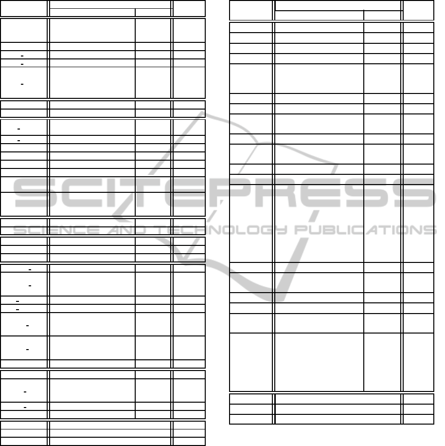
Table 8: The Best Results obtained by cBench.

CBR Best10

Program

Conﬁgurations Imp. (%) (%)

bitcount

AL.DF.AL.C, AL.DF.WE.C

AL.DF.AL.E, AL.DF.MI.E

AL.DF.WE.E

1.276 -45.748

qsort1

GR.DF.MI.C

10.958 6.709

susan c

RA.SF.AL.J

31.561 27.042

susan e

SA.DF.MI.C

4.279 1.862

susan s

SA.DF.AL.J, SA.DF.WE.J

SA.DF.AL.C, SA.DF.WE.C

SA.DF.AL.E, SA.DF.MI.E

SA.DF.WE.E

1.119 0.784

bzip2d

SA.DF.MI.J

20.796 39.972

bzip2e

RA.DF.MI.J

5.996 4.394

jpeg c

RA.DF.AL.J, RA.DF.MI.J

RA.DF.WE.J

11.436 5.686

jpeg d

RA.SF.AL.C, RA.SF.AL.E

8.086 4.894

lame

AL.SF.AL.J

7.554 8.748

mad

GR.SF.AL.J

2.038 1.303

tiff2bw

RA.DF.MI.E

16.784 7.449

tiff2rgba

SA.DF.MI.E

14.194 7.485

tiffdither

SA.DF.AL.J, SA.DF.WE.J

SA.DF.MI.C

-0.048 0.121

tiffmedian

RA.DF.MI.J, RA.DF.AL.C

RA.DF.WE.C, RA.DF.AL.E

RA.DF.WE.E

16.972 23.049

dijkstra

GR.DF.AL.J, GR.DF.WE.J

1.586 0.415

patricia

GT.DF.MI.E

0.321 0.562

ghostscript

SA.DF.MI.J

0.191 0.318

rsynth

RA.DF.MI.C

0.482 0.376

stringsearch1

RA.DF.MI.J, RA.DF.MI.E

-2.432 -18.242

blowﬁsh d

GR.DF.MI.E, GT.DF.MI.J

4.074 4.124

blowﬁsh e

GR.DF.MI.E, GT.DF.AL.J

GT.DF.MI.J

GT.DF.WE.J

4.053 3.943

pgp d

RA.SF.AL.J, RA.SF.AL.C

4.159 1.902

pgp e

SA.SF.AL.E

1.216 0.587

rijndael d

SA.DF.AL.C, SA.DF.WE.C

SA.DF.AL.E, SA.DF.MI.E

SA.DF.WE.E

13.125 0.003

rijndael e

SA.DF.AL.C, SA.DF.WE.C

SA.DF.AL.E, SA.DF.MI.E

SA.DF.WE.E

14.659 -2.211

sha

SA.DF.AL.J, SA.DF.WE.J

6.969 7.605

CRC32 *

2.126 2.126

adpcm c

AL.DF.AL.C, GT.DF.AL.C

GT.DF.WE.C, GT.DF.AL.E

GT.DF.WE.E

13.336 5.831

adpcm d

RA.SF.AL.J

16.96 11.183

gsm

SA.DF.AL.C, SA.DF.WE

1.609 1.967

API 7.593 3.656

APIE 8.202 6.412

NPI 29 28

the characteristic of a speciﬁc program, and not try to

cover several programs.

6.3 Coverage

The results shown in the previous section presented a

difﬁcult, in using a CBR approach to ﬁnd the best pre-

vious case that outperforms the well-engineered com-

piler level -O3, namely: it is necessary to try several

conﬁgurations. This is a problem, due to the high re-

sponse time. However, it is possible to use few con-

ﬁgurations and obtain good results.

Table 9: Best Results obtained by SPEC CPU2006.

CBR Best10

Program

Conﬁgurations Imp. (%) (%)

perlbench

AL.DF.MI.C, SA.DF.MI.C

12.926 10.138

bzip2

RA.DF.MI.C

6.882 7.280

gcc

GR.DF.MI.C

13.43 -2.929

mcf

RA.SF.AL.C, RA.SF.AL.E

10.128 9.307

milc

GT.DF.AL.J, GT.DF.WE.J

GT.DF.WE.C, GT.DF.MI.E

GT.DF.WE.E

3.49 -1.568

namd

AL.DF.MI.J, SA.DF.MI.J

5.582 4.928

gobmk

RA.DF.AL.J, RA.DF.WE.J

-0.176 -2.006

dealII

GR.DF.AL.J, GR.DF.MI.J

GR.DF.WE.J

-9.654 -4.262

soplex

AL.DF.MI.C

-0.174 0.376

povray

GR.DF.AL.E, GR.DF.MI.E

GR.DF.WE.E

0.485 0.679

hmmer

SA.DF.MI.E, RA.DF.MI.E

6.57 3.064

sjeng

SA.DF.MI.C, RA.DF.MI.C

6.75 5.495

libquantum

SA.DF.AL.J, SA.DF.MI.J

SA.DF.AL.C, SA.DF.MI.C

SA.DF.WE.C, SA.DF.AL.E

SA.DF.MI.E, SA.DF.WE.E

RA.DF.MI.J, RA.DF.AL.C

RA.DF.MI.C, RA.DF.WE.C

RA.DF.AL.E, RA.DF.MI.E

RA.DF.WE.E

19.287 19.126

h264ref

GT.DF.MI.C

1.825 -1.352

lbm

SA.SF.AL.C, SA.SF.AL.E

RA.SF.AL.C, RA.SF.AL.E

0.587 0.557

omnetpp

AL.SF.AL.J, GR.SF.AL.J

-1.303 -1.427

astar

GT.SF.AL.C, GT.SF.AL.E

3.062 -6.417

sphinx3

GT.DF.AL.J, GT.DF.MI.J

GT.DF.WE.J

13.99 12.811

xalancbmk

AL.DF.AL.C, AL.DF.MI.C

AL.DF.WE.C, AL.DF.AL.E

AL.DF.MI.E, AL.DF.WE.E

GR.DF.AL.C, GR.DF.MI.C

GR.DF.WE.C, GR.DF.AL.E

GR.DF.MI.E, GR.DF.WE.E

-1.719 -3.017

API 4.840 2.897

APIE 7.499 6.706

NPI 14 11

Using only three different conﬁgurations, it is pos-

sible to reach good results, without signiﬁcant loss of

performance. It is shown in Tables 10.

These results show a trade-off between perfor-

mance and response time. It means that the best per-

formance requires a high response time.

In cBench, it is necessary to tune several parame-

ters to reach good results. However, there is a loss of

performanceup to 22.10%. For cBench, it is difﬁculty

to reduce the variety of parameters. cBench needs at

least three different collections of previous cases, and

to use dynamic and static features.

In SPEC CPU2006, the system need to be tunned

only in the similarity model. For this benchmark, the

FindingGoodCompilerOptimizationSets-ACase-basedReasoningApproach

513

Table 10: Coverage Summary.

cBench

Restriction

Description

of the best

Group

APIE

Number

groups

No Restriction

RA.SF.AL.J

SA.SF.AL.E

AL.DF.MI.E

6.389 6

Only two Collections - - -

Only one Collection - - -

SPEC CPU2006

Restriction

Description

of the best

Group

APIE

Number

groups

No Restriction

RA.DF.MI.C

GR.DF.MI.E

GR.DF.MI.C

6.678 76

Only two Collections

RA.DF.MI.C

GR.DF.MI.E

GR.DF.MI.C

6.678 49

Only one Collection

GR.DF.MI.E

GR.DF.MI.C

GR.DF.MI.J

5.978 1

lost of improvement ranges from 10.95% to 20.28%.

In this benchmark, the reduced number of collections

is an excellent result, because this reduces the time

spent in the ofﬂine phase.

7 CONCLUSIONS AND FUTURE

WORK

Case-based Reasoning Approach. In this paper

we revisited the work of Lima et al., in oder to

explore new strategies of ﬁnding good compiler

optimization sets. The strategy is to create an

exploratory space that will be used by the Case-

based Reasoning approach to predict the compiler

optimization set, which should be enabled on an

unseen program.

Results. Our work indicate that if the main goal

is to ﬁnd the best conﬁguration that achieves the

best results, an interesting way it to use a random

strategy to build a collection of previous cases,

static features and Jaccard similarity model. On

the other hand, if the main goal is to cover more

programs, the use of dynamic features will be

more useful, and metaheuristics. The use of meta-

heuristics improves the covering range.

In our results, the random strategy was a good

choice to create a collection. Although, it was not

expected. It does not mean we do not have to use

metaheuristics to create collections. The results

indicate that the collection created by the genetic

algorithm with rank selector cover the maximum

programs of the SPEC CPU2006 benchmark.

It is possible to ﬁnd few conﬁgurations that

achieves a good performance. It reduces the time

spend in ofﬂineand online phases. However, there

is a trade-off between response time and perfor-

mance. Reducing the response time, in general,

decreases the average percentage improvement.

The CBR approach obtained good improve-

ments. It obtained an average percentage im-

provement of 4.84% for SPEC CPU2006, where

some programs achieved a improvement up to

10%. For cBench, the CBR obtained an aver-

age of 7.499%, where some improvements up to

15%. Besides, our CBR approach outperforms

the approach proposed by Purini and Jain, namely

Best10.

Critical Discussion. This work shows that it is dif-

ﬁcult to achieve performance based on only one

conﬁguration. Although, it is possible to achieve

a performance better than state-of-the-art algo-

rithms, it is necessary a high response time. Be-

sides, it is difﬁcult to achieve a good performance

for complex programs.

We should note that ﬁnding the best compiler

optimization set for a speciﬁc program, as deﬁned

by its input, is a problem without solution. There-

fore, the metric that we use is the best improve-

ment achieves by the best algorithm, presented in

the literature (the state-of-the-art).

The deﬁciency of all compiler optimizations or-

chestration strategies is to handle programs (train-

ing and test) as a black box. Programs are com-

posed by several different blocks. It indicates that

each block will probably be best optimized by a

speciﬁc compiler optimization set. It has to be in-

vestigated by new projects, in order to improvethe

state-of-the-art.

Future Work. We plan to propose new strategies

to characterize programs, new strategies to create

collections of previous cases, and new strategies

to select previous cases. In addition, we are inter-

ested in proposing a CBR approach that is able to

ﬁnd different previous cases for different parts of

the program.

ACKNOWLEDGEMENTS

The authors would like to thank CAPES for the ﬁnan-

cial support.

ICEIS2015-17thInternationalConferenceonEnterpriseInformationSystems

514

REFERENCES

Aamodt, A. and Plaza, E. (1994). Case-based reasoning;

foundational issues, methodological variations, and

system approaches. AI Communications, 7(1):39–59.

Aho, A. V., Lam, M. S., Sethi, R., and Ullman, J. D. (2006).

Compilers: Principles, Techniques and tools. Prentice

Hall.

cBench (2014). The collective benchmarks.

http://ctuning.org/wiki/index.php/CTools:CBench.

Access: January, 20 - 2015.

Cooper, K. and Torczon, L. (2011). Engineering a Com-

piler. Morgan Kaufmann, USA, 2nd edition.

Erbacher, R. and Hutchinson, S. (2012). Extending case-

based reasoning to network alert reporting. In Pro-

ceeding of the International Conference on Cyber Se-

curity, pages 187–194.

Henning, J. L. (2006). Spec cpu2006 benchmark de-

scriptions. SIGARCH Computer Architecture News,

34(4):1–17.

Jimenez, T., de Miguel, I., Aguado, J., Duran, R., Mer-

ayo, N., Fernandez, N., Sanchez, D., Fernandez, P.,

Atallah, N., Abril, E., and Lorenzo, R. (2011). Case-

based reasoning to estimate the q-factor in optical net-

works: An initial approach. In Proceedings of the Eu-

ropean Conference on Networks and Optical Commu-

nications, pages 181–184.

Kim, W., Baik, S. W., Kwon, S., Han, C., Hong, C., and

Kim, J. (2014). Real-time strategy generation system

using case-based reasoning. In Proceedings of the In-

ternational Symposium on Computer, Consumer and

Control, pages 1159–1162.

Lattner, C. and Adve, V. (2004). Llvm: A compilation

framework for lifelong program analysis & transfor-

mation. In Proceedings of the International Sym-

posium on Code Generation and Optimization, Palo

Alto, California.

Lima, E. D., De Souza Xavier, T., Faustino da Silva, A.,

and Beatryz Ruiz, L. (2013). Compiling for perfor-

mance and power efﬁciency. In Proceedings of the In-

ternational Workshop onPower and Timing Modeling,

Optimization and Simulation, pages 142–149.

LLVM Team (2014). The llvm compiler infrastructure.

http://llvm.org. Access: January, 20 - 2015.

Mendes, E. and Watson, I. (2002). A Comparison of

Case-Based Reasoning Approaches to Web Hyperme-

dia Project Cost Estimation. Proceedings of the Inter-

national Conference on World Wide Web, pages 272–

280.

Mitchell, T. M. (1997). Machine Learning. McGraw-Hill,

Inc., New York, NY, USA, 1 edition.

Mucci, P. J., Browne, S., Deane, C., and Ho, G. (1999).

Papi: A portable interface to hardware performance

counters. In Proceedings of the Department of De-

fense HPCMP Users Group Conference, pages 7–10.

Muchnick, S. S. (1997). Advanced Compiler Design and

Implementation. Morgan Kaufmann Publishers Inc.,

San Francisco, CA, USA.

Purini, S.and Jain, L.(2013). Finding good optimization se-

quences covering program space. ACM Transactions

on Architecture and Code Optimization, 9(4):1–23.

Richter, M. M. and Weber, R. (2013). Case-Based Reason-

ing: A Textbook. Springer, USA.

Shalev-Shwartz, S. and Ben-David, S. (2014). Understand-

ing Machine Learning: From Theory to Algorithms.

Cambridge University Press, Cambridge, USA.

Srikant, Y. N. and Shankar, P. (2007). The Compiler Design

Handbook: Optimizations and Machine Code Gener-

ation. CRC Press, Inc., Boca Raton, FL, USA, 2nd

edition.

Zhou, X. and Wang, F. (2014). A spatial awareness case-

based reasoning approach for typhoon disaster man-

agement. In Proceedings of the IEEE International

Conference on Software Engineering and Service Sci-

ence, pages 893–896.

Zhou, Y.-Q. and Lin, N.-W. (2012). A Study on Optimizing

Execution Time and Code Size in Iterative Compila-

tion. Third International Conference on Innovations

in Bio-Inspired Computing and Applications, pages

104–109.

FindingGoodCompilerOptimizationSets-ACase-basedReasoningApproach

515