Convex Hull Brushing in Scatter Plots

Multi-dimensional Correlation Analysis

Miguel Nunes, Kresimir Matkovic and Katja B

uhler

VRVis Research Center, Vienna, Austria

Keywords:

Visual Analytics, Convex Hull Brush, Scatter Plots, Linked Views, Correlation.

Abstract:

Interactive Visual Analysis has been widely used for the reason that it allows users to investigate highly

complex data in coordinated multiple views, showing different perspectives over data. In order to relate data,

multiple techniques of brushing have been introduced. This work extends the state of the art by introducing

the Convex Hull (CH) Brush, which is a new way of selecting and interpreting high dimensional data in scatter

plot (SP) views. By using a combination of brushes through linked views, the CH-Brush allows the selection

and clustering of values that are not typically deﬁned by SP ranges, in spite of sharing similarities. In CH-

Brushing is also able to visually report the existence of correlation between variables. Furthermore, we discuss

CH-Brushing sensitivity and the application of smoothness. We use synthetic data to support our rationale and

clarify the intrinsic meanings of CH-Brushing in scatter plots. We also report on the ﬁrst experience on using

the CH-Brush in a real-world medical case.

1 INTRODUCTION

Through Interactive Visual Analysis (IVA), a range

of linked views displaying different data visualiza-

tion techniques is available for visual inspection

of relations between variables of complex datasets.

It is consistently used in numerous ﬁelds such as

science (Mart

ınez-G

omez et al., 2014), engineer-

ing (Sedlmair et al., 2011) or ﬁnance (Inselberg,

2009) for hypothesis generation, evaluation and sense

making. According to task and domain of the

data, different visualization methods can be com-

bined. These include scientiﬁc visualization, statisti-

cal graphics and computational tools (Konyha et al.,

2006) which are used to uncover hidden informa-

tion in multi-dimensional datasets by making use of

human intuition and respective domain knowledge

for data analysis. It is through coordinated multi-

ple views (Roberts, 2007) that users are able to com-

pare different values, perspectives or interpretations

of data.

The scatter plot is one of the most often used

views in data visualization and has been extensively

studied (Li et al., 2010; Rensink and Baldridge,

2010). Scatter plots are often used to visually de-

termine existence of clusters in data and respective

correlations between two variables. However, often

times is not feasible for users to fully visualize and

understand complex clusters of points when a high

number of variables are being analysed. Relationship

between variables become harder to visually inspect

when hundreds or thousands of data points are plot-

ted in coordinated multiple views. Convex hulls have

been used in scatter plots to support the construction

of convexity measures (Wilkinson et al., 2006) and to

allow navigation and query sculpting in scatter plots

matrices (Elmqvist et al., 2008).

Obtaining clusters from convex hulls was al-

ready achieved (Sainath et al., 2011; Pratt et al.,

2014) showing how they can be generically applica-

ble (Wilderjans et al., 2013). A review on literature

about methods and techniques for clustering (Estivill-

Castro, 2002) shows how well developed this ﬁeld of

research is. However, it is argued that different algo-

rithms may not run in the same datasets, forcing users

to be aware of the best method for each case. Through

IVA, composite brushing and Convex Hull brushing,

we believe users may obtain clusters and respective

information in a visual and intuitive manner.

To enable CH-brushing and to support analysis

and visualization tasks in coordinated multiple views,

navigating between overview and detail of datasets is

fundamental. Typically, this is achieved by brushing,

which is an important tool for visually inspecting data

in an interactive manner. Brushing in one linked view

highlights subsets of data displayed in other linked

182

Nunes M., Matkovic K. and Bühler K..

Convex Hull Brushing in Scatter Plots - Multi-dimensional Correlation Analysis.

DOI: 10.5220/0005356501820189

In Proceedings of the 6th International Conference on Information Visualization Theory and Applications (IVAPP-2015), pages 182-189

ISBN: 978-989-758-088-8

 2015 SCITEPRESS (Science and Technology Publications, Lda.)

Table 1: Details of synthetic datasets.

Dataset ID Dimensions Data Points

1 7 300

2 10 500

3 13 300

4 6 1550

5 4 1500

6 4 1000

7 6 500

8 7 680

views, facilitating the understanding of relationships

between a high number of variables. This iterative

and interactive process of brushing in different con-

nected views, allows information drill-down where

previously selected data points become the new focus

of analysis, enabling further brushing in a sub-context

of the data. It is also possible to use a combination of

multiple brushes across linked views to extract mul-

tiple features or discover patterns in data (Martin and

Ward, 1995; Roberts, 2007). Respective selected data

points are highlighted in the respective brush’s colour.

The CH-Brush is different from typical brushing since

the brush range selection is no longer the user’s re-

sponsibility, but is automatically created by taken in

consideration linked data points originated from com-

posite brushing in other linked views.

The major contribution of this work is the intro-

duction of Convex Hull Brush in scatter plots. We dis-

cuss what are the implications and interpretations of

combining linked brushing with CH-Brush in linked

views. In addition, we also consider the potential of

including a smoothness factor (Doleisch and Hauser,

2002) for CH-Brushes, together with an interpretation

of brush sensitivity and how to tackle such issue with

smooth brushing. Multidimensional datasets from an

online data repository and a real medical case were

used in this work.

2 DATA

To support the reasoning behind the use of the CH-

Brush, we used 8 synthetic datasets that were ex-

plored by means of a coordinated multiple views sys-

tem (Matkovic et al., 2008). The system supports par-

allel coordinates (PC), histograms and scatter plots.

Synthetic datasets were obtained from an open

data generator, Sketchpad N-D (Wang et al., 2013),

with dimensions ranging from 4 to 13 variables. The

number of points present in these datasets ranged

from 300 to 1550. Table 1 shows details about each

dataset. None of our datasets was targeted with di-

mension reduction techniques, nor were they previ-

Figure 1: Parallel Coordinates obtained in Sketchpad N-D

while generating dataset 8 with manually set probability

density functions and quadrilateral data connection.

ously classiﬁed. We used the original dimensions and

data points delivered by the synthetic data generator.

Figure 1 depicts the generated PC for dataset 8 in

Sketchpad N-D. It can be seen that six probability

density functions were set to create clusters and one

quadrilateral data connection was added between the

last two axes.

3 BRUSHING IN SP

Introduced more than 25 years ago (Becker and

Cleveland, 1987; Fisherkeller et al., 1988), brush-

ing in scatter plots became one of the most com-

mon methods for displaying and interacting with

multi-dimensional data in the information visualiza-

tions scope. Scatter plots relate two dimensions of a

dataset and, together with other linked scatter plots or

other views, many variables of a dataset can be vi-

sually assessed at the same time in a straightforward

way (Sedlmair et al., 2013).

Brushing in scatter plots is routinely done by se-

lecting a cross-section of two ranges, which is visu-

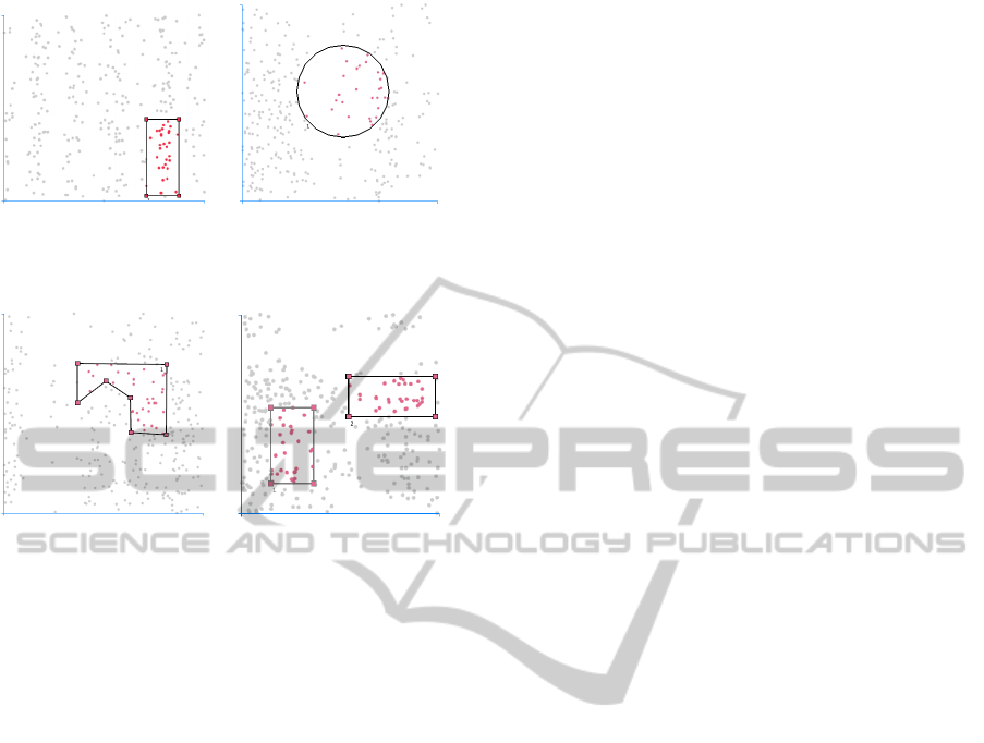
ally represented by a rectangular box (Figure 2 (a)).

Other forms of brushing in scatter plots include, but

not limited to, circular brushes (Figure 2 (b)) and

lasso brushes (Figure 3 (a)), which gives ﬂexibility on

how users select ranges in scatter plots. Data relations

within Circular brushes are hard to interpret if units

and scales of parameters are different. Brushed data

points will be inside a circular area around a point. As

for lasso brushes, these have more complicated inter-

pretations but are used for selection of complex sub-

sets. It is also possible to obtain complex subsets by

using a composite brushing where brushes are be log-

ically combined (Figure 3 (b)).

Figures 4 (a) and (b) show two linked scatter plots.

Data from dataset 3 is plotted so variables M, E and I

can be used for brushing and analysis. After plotting

data in both linked scatter plots, a box brush is created

which selects data points for M and E axes (Figure 4

(a). While brushing the ﬁrst scatter plot data points, in

ConvexHullBrushinginScatterPlots-Multi-dimensionalCorrelationAnalysis

183

(a) (b)

Figure 2: Examples of a Box Brush (a) and of a Circle Brush

(b) in 2D Scatter Plots.

(a) (b)

Figure 3: Example of a Lasso Brush in a 2D Scatter Plot (a)

and a composite brush of Box Brushes selecting different

ranges (b).

the second scatter plot (Figure 4 (b)) the correspond-

ing linked points get highlighted with the same colour.

However, since the second scatter plot is comparing

two other dimensions of the dataset, which have dif-

ferent ranges and distribution of values, these points

do not visually correspond to the same area as in the

ﬁrst scatter plot.

As such, brushing in coordinated multiple views

systems introduces two terms to deﬁne data points:

brushed data and linked data. The ﬁrst one deﬁnes

data points that are inside the area of a brush, as seen

in Figures 2 and 3. Linked data are data points that

have been brushed in one view, but are displayed in

another view relating other dimensions of the dataset

(Figure 4 (b)). These data points are highlighted with

the same colour as the brush that originally selected

them. Brushed data and linked data will later be used

to help deﬁne the CH-Brush.

To facilitate the deﬁnition of a gradual change

between brushed data and not brushed data, and to

avoid the sudden tumble present in binary brushes’

edges, smoothness enhances the focus+context work-

ﬂow by applying a degree of continuity between 1 and

0 to surrounding data points (Oeltze et al., 2012). It

supports users in discerning a degree of interest over

brushed data. An example is the deﬁnition of a range

of opacity values to depict ﬂow in volume render-

ing (Doleisch et al., 2003).

Smooth brushing can also be used to extract mean-

ing from neighbouring data points that have simi-

lar characteristics to the ones inside the brushed re-

gion. Applying a smoothness factor to a brush has

the power to elucidate expert users about properties of

data points that were not initially selected. Depending

on the context, these properties can range from corre-

lation of selected data points and signature similarities

to uncertainty.

Brush sensitivity can be seen as how much linked

data changes when a brush is changed. If a small

change in the brush (e.g.: panning, resizing) results

in a large change over linked data, then the brush can

be considered very sensitive, otherwise it has low sen-

sitivity. The sensibility of brushes should always be

evaluated by the domain expert in its corresponding

context. Smooth brushing can then be used to guar-

antee that the brush is not placed in a highly sensitive

range.

4 THE CONVEX HULL BRUSH

Parallel Coordinates, for example, are a good method

to ﬁnd patterns and certain clusters of information.

However, the selection of values in PC are translated

to SP as rectangular brushes. Trying to do so, would

most probably incur in adding data points that would

not be taken into consideration by the convex hull

algorithm. We will introduce now the Convex Hull

brush which overcomes this problem.

For any subset of points in a 2D plane, its convex

hull is the smallest convex polygon that contains that

subset. So, for the case of creating a CH-Brush in

a scatter plot, all linked data points brushed in other

linked views will be used for the construction of the

convex hull, together with points that were not se-

lected but are inside of the 2D subset.

In cases where visual clusters arise by (more or

less complex) brushing, existing brushes are not able

to efﬁciently and quickly gather all points inside the

originally brushed subset. The addition of the CH-

Brush quickly overcomes this issue. The CH-Brush

facilitates this process by geometrically analysing the

linked data points and creating a convex hull around

the previously selected data points, automatically cre-

ating a cluster which can then be focused on and anal-

ysed. As an example to illustrate this, a scatter plot

gets set up and data points get brushed (Figure 4 (a)).

As a result, in another linked scatter plot, comparing

two other variables of the same dataset, linked data

points get highlighted (Figure 4 (b)) with the colour

of the original brush. Only then, the creation of a CH-

Brush becomes possible. Because there is linked data

IVAPP2015-InternationalConferenceonInformationVisualizationTheoryandApplications

184

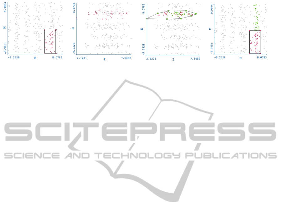
(a) (b) (c) (d)

Figure 4: Scatter plot with brushed data (a) and respective highlighted linked data in a second Scatter Plot (b). Automatically

created Convex Hull brush from linked data (c). Original scatter plot displaying new green linked points as a result of creating

a Convex Hull brush (d).

highlighted, the generation of a convex brush hull of

those linked points is a quick operation and results

in a new brush, with a new colour, selecting all data

points inside of it (Figure 4 (c)).

Following the same logic, these new brushed data

points (in green) will then be highlighted in the pre-

vious linked scatter plots, giving instant information

about how many new data points got brushed, as seen

in Figure 4 (d). From the differences found in the

quantity of brushed data points and the size of the CH-

Brush, different conclusions about data points and

variables can be reached.

4.1 Interpretations

Generating a convex hull in a scatter plot can help

disclose properties of the brushed data. Furthermore,

including a smooth region to the CH-Brush allow

users investigating its sensitivity. The result of CH-

Brushing can help:

• to verify how much correlation exist between the

two variables plotted in the SP (M1),

• to verify how similar the newly added points are

in relation to previously selected data points (M2),

• to check for the existence of clustering data points

(M3),

• to contextualize data points that were not initially

selected (M4).

Correlation between variables (M1) can be vi-

sually obtained by brushing ranges of data points

of interest and later visualized across linked views

of plotted data. Yet, when users are dealing with

datasets containing dozens of variables and thousands

of points, such task can eventually become higher in

complexity and prone to human error due to clutter

of information and time spent in focus+context sub-

tasks. Correlation can be intuitively visualized by

analysing the size of the CH-Brush in relation to the

total of data points spread in the SP. If the CH-brush

focus in a small area of the SP, it can be concluded that

a correlation exists between the two plotted variables,

in relation to the brushed data points. Otherwise, se-

lected data points hold little correlation between se-

lected data points.

Gathering data points by applying a CH-Brush in

a SP after users brush and focus+context will return

points with similar characteristics. Users can then es-

timate how meaningful the newly added data points

are in comparison to the originally brushed points

(e.g., following the same trend, having similar rela-

tions to other variables).

Clustering of highly complex data has been

broadly studied and many methods have been eval-

uated. By introducing the CH-Brush, we propose a

visual check of clusters by making use of IVA (M3).

Keeping in mind points (M1) and (M2), by creating

a CH-Brush over previously brushed linked data, it

is possible to check clustering in other dimensions.

A good example of this would be the case where

a multi-dimensional dataset consisting of clusters of

data could be well represented and easily brushed in a

linked view where two variables are compared. How-

ever, the same cluster would be hard to distinguish by

using different variables. Generating the CH-Brush

would easily select all points previously selected to-

gether with data points inside the CH-Brush. (M1)

and (M2) could then be used to assess how well these

two new variables can be used for further clustering

of data, focus and contextualization.

IVA allows visualizing data in different paradigms

(e.g.: volume rendering) which can contribute to a

better understanding of the extent of the CH-Brush

(M4). By (M1), (M2) and (M3) users are given

the possibility to evaluate and contextualize all data

points inside the CH-Brush and how well they cor-

relate or cluster. In Section 5, we use the results of

linked brushing and CH-brushing in scatter plots to

further clarify the intrinsic meaning of these 4 points.

ConvexHullBrushinginScatterPlots-Multi-dimensionalCorrelationAnalysis

185

Figure 5: Example of a Convex Hull Brush with a smooth-

ness factor in a 2D Scatter Plot. Points inside smooth area

are highlighted with a faded colour of the brush.

4.2 CH-Brush Sensitivity

We deﬁne sensitivity of the CH-Brush differently as

reported in Section 3. When generating a new CH-

Brush, two things can happen: no extra data points

are included or new data points are included. For

the ﬁrst case, sensitivity is null since no changes in-

curred. This supports on saying that, for the origi-

nally brushed data points, total correlation exist be-

tween the two variables plotted in the SP (M1).

On the other hand, if new data points are included

in the CH-Brush, several possibilities arise. If a high

percentage of data points are included, we can say

that the sensitivity of the CH-Brush is very high, for

it changes much of the linked data. This can also be

an indication of low correlation between plotted vari-

ables (M1). If the data points selected by the CH-

Brush present similarities to other data points in other

linked views (e.g.: the same pattern in PC) the brush

has low sensitivity. An example of this can be seen

in Figure 4 (c) where red points belong to the original

brush and green points are the points selected by the

CH-brush.

Including a smoothness factor (Figure 5) impacts

the sensibility of the brush as data points that were not

initially inside the CH-Brush might be included. This

addition can check if near-by data points also have

correlation to the data points inside the CH-Brush

(M1), verify if these points belong to the same or sim-

ilar context of brushed data points (M2 and M4) and,

ﬁnally, check how these data points in the smooth re-

gion might integrate a cluster (M3).

4.3 Implementation

Our implementation of the CH-brush is based on An-

drew’s monotone chain convex hull algorithm (An-

drew, 1979). All brushed data points from the data

table are taken in consideration to build the convex

hull. After the user brushes a series of ranges across

dimensions of a dataset in one or more linked views

using one or more brushes, s/he can investigate in a

scatter plot how two dimensions relate. In case new

data points are selected after the CH-Brush is gener-

ated, and because all views are linked, it is possible to

immediately see the effect of how the linked data gets

changed/highlighted.

We incorporated smooth brushing in our CH-

brush in order to allow inspection of uncertainty and

also deal with brush sensitivity. Smoothness is seen

as an outside doted contour (Figure 5) that is created

by ﬁrst calculating the centroid of the CH-brush, next

calculating the vectors of the centroid to each vertex

of the CH-Brush and then applying a smoothness fac-

tor to each vector. This creates the vertices of the CH-

brush’s smoothness line. Points inside the smoothness

area are given values between 0 and 1.

To actually create the CH-brush, the user has to

select values from a data table using available linked

views. After values are selected, a scatter plot dis-

playing selected linked points should be made avail-

able to allow the creation of the CH-Brush. In our

prototype, to create it, the user only has to click the

option for Convex Hull Generation. Immediately, a

lasso brush is calculated gathering the linked points

in that view space, by means of the convex hull algo-

rithm. As soon as the brush is created, all other views

are updated with the newly selected values with the

respective CH-brush colour.

5 RESULTS AND DISCUSSION

Linked views were used to analyse, brush and com-

pare our synthetic and real datasets (Section 2). Since

our synthetic datasets did not contain more then 1550

samples, visual recognition of clusters and correla-

tions between certain dimensions were usually easily

achieved. We make use of the CH-Brush to reach the

same observations.

5.1 Dataset 4

For dataset 4, we started by plotting values of vari-

able B in a histogram, and brushed a single bin with a

red brush (Figure 6 (a)). We then plotted in a scatter

plot the values of A and C. It was noticeable that both

variables had a certain degree of local correlation for

the brushed data points of B. We then created a CH-

Brush, as seen in Figure 6 (b)) for those linked data

points and realized that the histogram in Figure 6 (a)

displayed extra selected data points all across dimen-

sion B.

IVAPP2015-InternationalConferenceonInformationVisualizationTheoryandApplications

186

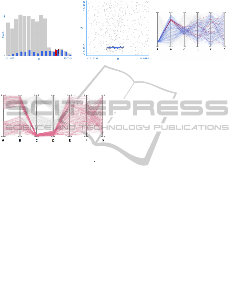
(a) (b) (c)

Figure 6: Linked histogram view plotting values of B from dataset 4. Red values selected from red brush and blue values

selected by blue CH-brush (a). Linked SP view plotting values of A and C from dataset 4 with a CH-Brush (b). Resulting PC

linked view showing local correlation between variables A and C from dataset 4 (c).

Figure 7: Parallel Coordinates overview of dataset 8.

We then plotted all dimensions of dataset 4 in a

linked PC view (Figure 6 (c)). We were able to ob-

serve the relationship between all variables and anal-

yse the level of correlations between A, B and C. It

is easy to observe that, for the selected range of B in

red, a very small range of A is selected, showing high

correlation between these two variables (M1). How-

ever, such a high degree of correlation is not noted

between B and C. Actually, the creation of the CH-

Brush shows that many values of B get selected (M2),

and that these values have very little correlation to

variable C. Yet, it is still possible to observe that, for

the newly range of C values, there is a high degree of

local correlation with A (M3).

5.2 Dataset 8

Dataset 8 was purposely built in a way that some vari-

ables are highly correlated while others have no cor-

relation at all. By visually inspecting the PC view

of dataset 8 (Figure 7), it is visually perceptible that

variables A and B, and C and D are highly correlated,

while variables E, F and G have no apparent correla-

tion.

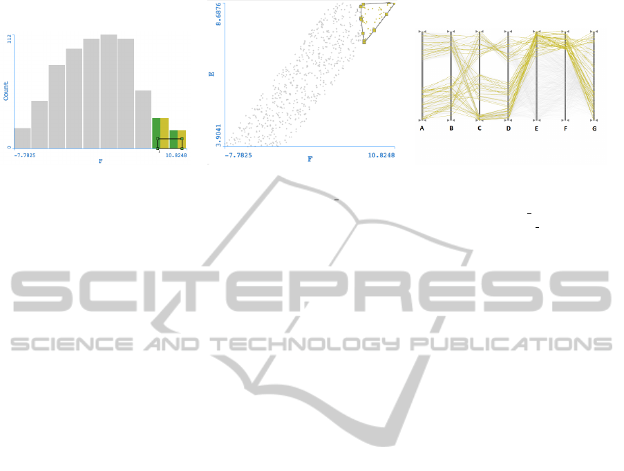
Next, by brushing high values of F, we were able

to see that there was, in fact, a local correlation be-

tween E and F (M1). Figure 8 (a) shows the high val-

ues of F brushed in green, while Figure 8 (b) depicts

the generated CH-Brush in a scatter plot comparing E

to F. It can then be seen in the PC view that variables

E and F have a certain correlation for high values of

F (Figure 8 (c)). Also, Figure 8 (b) shows that no ex-

tra values of F were selected by the CH-Brush (green

colour), pointing in the direction that these brushed

data points form a cluster (M3). Observing the result-

ing PC and histogram we can see no extra data points

are selected by the CH-Brush. This is a special case of

the CH-Brush that, when correlation is total, the same

operation could be performed by simply brushing the

same ranges in the PC.

5.3 An Example with Medical Data

Datasets from an ongoing project, where we closely

collaborate with medical experts (Nunes et al., 2014),

were composed of between 7 and 12 variables

and number of points ranging between 35.000 and

550.000. These variables correspond to medical im-

ages such as Magnetic Resonance (MR) T1-weighted,

molecular components of MR Spectroscopy Imag-

ing (MRSI), manual segmentations and X, Y, Z co-

ordinates of patients with brain cancer. Following

medical guidance, three more dimensions relating

three molecular components through their ratios were

added to the datasets.

An initial version of the CH-Brush was used to

answer a real medical need. Magnetic Resonance

Spectroscopy Imaging (MRSI) was evaluated in an

IVA system connecting a Visual Analytics system to

a medical imaging framework, which allowed doc-

tors to analyse MRSI data in an intuitive and ﬂexi-

ble manner for the ﬁrst time. By plotting MRSI val-

ues in linked views, and using multiple brushes, pat-

terns arouse and there was a need to create clusters

of data. CH-Brushing gathered extra 3D MRSI vox-

ConvexHullBrushinginScatterPlots-Multi-dimensionalCorrelationAnalysis

187

(a) (b) (c)

Figure 8: Linked histogram view plotting values of F from dataset 8. Values in green are brushed from the green brush.

Yellow values originate from CH-Brushing (a). Linked SP view plotting values of E and F from dataset 8 with a yellow

CH-Brush (b). Resulting PC linked view showing local correlation between variables E and F from dataset 8. Yellow and

green lines are overlapped (c).

els that were not previously taken into account by the

doctors segmentations. It was found that data points

included in the CH-Brush had correlation (M1) and

presented very similar signatures as segmented vox-

els (M2). By visually inspecting the newly selected

voxels in anatomical rendering, it was noted that 3D

voxels bordering the original segmentation were high-

lighted (M4). These results point in the direction that,

by using IVA, a better understanding about cancer

can be achieved, to ultimately design better treatment

plans for patients.

It was also observed that the CH-Brush selected

values that corresponded to very speciﬁc and sparse

ranges in PC. This goes in line to what was indicated

in Section 4 that brushing a range in a PC axis is the

same as creating a rectangular brush in a SP and does

not allow ﬂexibility in this sort of cluster discovering.

The CH-Brush overcame this issue.

The examples and results herein presented and

discussed show the potential of using CH-Brushing

for clustering, contextualizing and correlation ﬁnd-

ing. Synthetic datasets and one real world case sup-

port our initial hypothesis (M1–M4) that CH-Brushes

can positively impact the way users interact and anal-

yse multi-dimensional datasets in scatter plots.

6 LIMITATIONS AND FUTURE

WORK

We understand that there are datasets that might

not follow the patterns and clustering presented

here (Sedlmair et al., 2013). As such, an alterna-

tive to the CH-Brush could be a Concave Hull Brush

from where similar meanings could be extracted from,

but where brushed data is presented in a way that

would not be meaningful while employing a CH-

Brush (Moreira and Santos, 2007).

Another key point for further CH-Brush valida-

tion would be to extend its applicability into more

real world multi-dimensional datasets. A proper eval-

uation of the performance of this brush with the re-

spective domain experts will certainly add value and

better deﬁnitions for this brush. Also, using CH-

Brushing with SP matrices would further enlighten

the true power of the presented brush.

Lastly, smoothness in CH-Brush can be alterna-

tively approached. Another way we can envision the

construction of the smoothness region would be to

sample neighbouring points from the original CH-

Brush’s vertices, and then use these new points to

create a new CH-brush region. This, and other al-

ternatives, would have to be properly evaluated and

compared in order to assess the respective usefulness,

not only as a general application but also in speciﬁc

domains.

7 CONCLUSIONS

This work introduced a new way of brushing for IVA.

We used linked views and a rendering system to vi-

sualize linked brush data and analyse the result of

including Convex Hull brushing. Synthetic multi-

dimensional datasets were used to show the general

applicability of the CH-Brush as well as real data

from medical studies.

Our approach suggests that CH-Brush can be use-

ful for cases where interpretation of data inside clus-

ters might not be trivial. Also, we consider that visu-

ally inspecting the existence of clusters and relation-

ships between high number of variables is simpliﬁed.

IVAPP2015-InternationalConferenceonInformationVisualizationTheoryandApplications

188

ACKNOWLEDGEMENTS

The authors wish to thank the reviewers for their care-

ful reading of the manuscript and helpful comments.

This work is part of the SUMMER Marie Curie Re-

search Training Network (PITN-GA-2011-290148),

which is funded by the 7th Framework Programme

of the European Commission (FP7-PEOPLE-2011-

ITN). The centre of excellence, VRVis, is ﬁnanced by

COMET – Competence Centers for Excellent Tech-

nologies by BMVIT, BMWFJ and ZIT – The Tech-

nology Agency of the City of Vienna. The COMET

Programme is managed by FFG.

REFERENCES

Andrew, A. M. (1979). Another efﬁcient algorithm for con-

vex hulls in two dimensions. Information Processing

Letters, 9(5):216–219.

Becker, R. A. and Cleveland, W. S. (1987). Brushing scat-

terplots. Technometrics, 29(2):127–142.

Doleisch, H., Gasser, M., and Hauser, H. (2003). Inter-

active feature speciﬁcation for focus+ context visual-

ization of complex simulation data. In Proceedings

of the symposium on Data visualisation 2003, pages

239–248. Eurographics Association.

Doleisch, H. and Hauser, H. (2002). Smooth brushing for

focus+context visualization of simulkation data in 3d.

Elmqvist, N., Dragicevic, P., and Fekete, J.-D. (2008).

Rolling the dice: Multidimensional visual explo-

ration using scatterplot matrix navigation. Visualiza-

tion and Computer Graphics, IEEE Transactions on,

14(6):1539–1148.

Estivill-Castro, V. (2002). Why so many clustering algo-

rithms: A position paper. SIGKDD Explor. Newsl.,

4(1):65–75.

Fisherkeller, M. A., Friedman, J. H., and Tukey, J. W.

(1988). Prim-9: An interactive multi-dimensional data

display and analysis system. In In Dynamic Graphics

for Statistics, pages 111–120.

Inselberg, A. (2009). Parallel coordinates. Springer.

Konyha, Z., Matkovic, K., Gracanin, D., Jelovic, M., and

Hauser, H. (2006). Interactive visual analysis of fam-

ilies of function graphs. Visualization and Computer

Graphics, IEEE Transactions on, 12(6):1373–1385.

Li, J., Martens, J.-B., and Van Wijk, J. J. (2010). Judging

correlation from scatterplots and parallel coordinate

plots. Information Visualization, 9(1):13–30.

Martin, A. R. and Ward, M. O. (1995). High dimen-

sional brushing for interactive exploration of multi-

variate data. In Proceedings of the 6th Conference on

Visualization’95, page 271. IEEE Computer Society.

Mart

ınez-G

omez, E., Richards, M. T., and Richards, D. S. P.

(2014). Distance correlation methods for discovering

associations in large astrophysical databases. The As-

trophysical Journal, 781(1):39.

Matkovic, K., Freiler, W., Gracanin, D., and Hauser, H.

(2008). Comvis: A coordinated multiple views sys-

tem for prototyping new visualization technology. In

Information Visualisation, 2008. IV ’08. 12th Interna-

tional Conference, pages 215–220.

Moreira, A. and Santos, M. Y. (2007). Concave hull: A

k-nearest neighbours approach for the computation

of the region occupied by a set of points. Proceed-

ings of the 2nd International Conference on Computer

Graphics Theory and Applications.

Nunes, M., Rowland, B., Schlachter, M., Ken, S., Matkovic,

K., Laprie, A., and B

uhler, K. (2014). An integrated

visual analysis system for fusing mr spectroscopy and

multi-modal radiology imaging. In Proceedings of

IEEE VAST 2014.

Oeltze, S., Doleisch, H., Hauser, H., and Weber, G. (2012).

Interactive visual analysis of scientiﬁc data. Tutorial

at the IEEE VisWeek 2012.

Pratt, J., Busse, A., Mueller, W.-C., Chapman, S., and

Watkins, N. (2014). Anomalous dispersion of la-

grangian particles in local regions of turbulent ﬂows

revealed by convex hull analysis. arXiv preprint

arXiv:1408.5706.

Rensink, R. A. and Baldridge, G. (2010). The perception

of correlation in scatterplots. volume 29, pages 1203–

1210. Wiley Online Library.

Roberts, J. C. (2007). State of the art: Coordinated & mul-

tiple views in exploratory visualization. In Coordi-

nated and Multiple Views in Exploratory Visualiza-

tion, 2007. CMV’07. Fifth International Conference

on, pages 61–71. IEEE.

Sainath, T. N., Nahamoo, D., Kanevsky, D., Ramabhad-

ran, B., and Shah, P. (2011). A convex hull ap-

proach to sparse representations for exemplar-based

speech recognition. In Automatic Speech Recognition

and Understanding (ASRU), 2011 IEEE Workshop on,

pages 59–64. IEEE.

Sedlmair, M., Isenberg, P., Baur, D., Mauerer, M., Pigorsch,

C., and Butz, A. (2011). Cardiogram: visual analyt-

ics for automotive engineers. In Proceedings of the

SIGCHI Conference on Human Factors in Computing

Systems, pages 1727–1736. ACM.

Sedlmair, M., Munzner, T., and Tory, M. (2013). Empirical

guidance on scatterplot and dimension reduction tech-

nique choices. Visualization and Computer Graphics,

IEEE Transactions on, 19(12):2634–2643.

Wang, B., Ruchikachorn, P., and Mueller, K. (2013).

Sketchpadn-d: WYDIWYG sculpting and editing in

high-dimensional space. CoRR, abs/1308.0762.

Wilderjans, T. F., Ceulemans, E., and Meers, K. (2013).

Chull: A generic convex-hull-based model selection

method. Behavior research methods, 45(1):1–15.

Wilkinson, L., Anand, A., and Grossman, R. (2006). High-

dimensional visual analytics: Interactive exploration

guided by pairwise views of point distributions. Visu-

alization and Computer Graphics, IEEE Transactions

on, 12(6):1363–1372.

ConvexHullBrushinginScatterPlots-Multi-dimensionalCorrelationAnalysis

189

REFERENCES

Andrew, A. M. (1979). Another efficient algorithm for con-