
Ensuring Blood is Available When it is Needed Most
Nigel M. Clay, John W. Hearne, Babak Abbasi and Andrew Eberhard
School of Mathematics and Geospatial Science, RMIT University, Bourke Street, Melbourne, Australia
1 STAGE OF THE RESEARCH
This research is in the first year of a three to four
year program. An initial review of the literature has
been undertaken and, as this document will show, an
approach is proposed to address the research ques-
tions. Some initial work has commenced using this
approach but much more will be required for comple-
tion.
2 OUTLINE OF OBJECTIVES
There are several objectives of this research:
• To establish a mathematical basis for the variance
seen in real blood inventory data;
• To develop a blood inventory simulation model
which incorporates this mathematical basis;
• To compare the outcome of the simulation model
with competing models of blood inventory;
• To use the model to analyse the impact of alter-
native blood inventory policies on the supply of
blood.
3 RESEARCH PROBLEM
Past research conducted into the management and be-
haviour of blood inventories relies on distributional
assumptions regarding the supply and demand for
blood which tend to underestimate the true variation
in inventory volumes. This may lead to the underesti-
mation of blood shortages and outdates and/or give a
false sense of security to inventory managers. This re-
search will address this issue from a mathematical and
modelling perspective and will use the results to ex-
amine the impact of alternative blood inventory poli-
cies.
It is hypothesised that variation in blood invento-
ries arises from two canonical sources. Firstly, the
process of donation, storage, hospital orders, supply
and transfusion consists of delays at several points.
These delays can cause system oscillation and insta-
bility as a result of small changes in demand with-
out the presence of stochastic variation in demand and
supply.
The second source of variation is the stochastic
nature of demand and supply themselves. When con-
sidered together with the first source of volatility the
total variation in the system may be amplified.
It is believed that a model incorporating both of
these sources of variation will exhibit the degree of
volatility seen in the real data. Such a model could
then be used to optimise inventory decisions or test
the behaviour of the inventory to potential changes in
blood storage, donor behaviour and so forth.
4 STATE OF THE ART
4.1 Early Work
The science of inventory management can be traced
back to 1913 when the first derivation of the economic
order quantity was given (Harris, 1913). This initial
work went substantially unchanged until 1951 when
an optimal solution to the (s, S) inventory policy was
presented (Arrow et al., 1951).
This seminal work assumed that the commodity
could be re-ordered at specific intervals and incorpo-
rated uncertainty in demand. The inventory manager
chooses two values, S and s, where S > s. If the inven-
tory on hand, y
t
, at time t is less than s then the inven-
tory manager orders S−y
t
of the commodity from the
supplier to meet future demand. The problem faced
by the inventory manager is to choose suitable val-
ues of S and s that are optimal in the sense that they
minimise the combined cost of holding the stock and
placing an order. Arrow et al. provided an optimal
solution to this problem.
However, other inventory policies could also be
used by an inventory manager. Instead of an (s, S)
policy a manager could take other approaches. For ex-
ample, he could replace the commodity as soon as it
was ordered, he could make few but large orders or he
3
M. Clay N., Hearne J., Abbasi B. and Eberhard A..
Ensuring Blood is Available When it is Needed Most.
Copyright
c
2015 SCITEPRESS (Science and Technology Publications, Lda.)

could make frequent small orders. How could a man-
ager be certain that choosing an optimal (s, S) policy
was superior to these alternatives? It turns out that
where demand is uncertain the optimal (s, S) policy
is optimal over any alternative inventory policy that
could be adopted (Scarf, 1960) although the proof was
not available until several years after the paper from
Arrow et.al.
4.2 Perishable Inventory
Some commodities have a fixed life span. We might
immediately think of such things as milk, eggs, bread
and so on but there are other examples: photographic
material, chemical weapons in a store, some short half
life radioactive items. If demand were known with
certainty for these then it would be easy to order in
such a way that the commodity never perishes. The
combination of demand uncertainty and a perishable
(fixed-lifetime) commodity is a more challenging one
than one where the demand is uncertain but the com-
modity has an infinite lifetime.
This forces us to confront not just the optimal or-
der polices in the face of uncertain demand but the
optimal issuing policies as well. The two ends of the
continuum for these are first in first out (FIFO) and
last in first out (LIFO). It seems fairly intuitive that a
FIFO policy is optimal for such inventories and early
proofs for some simple cases were provided in 1958
(Derman and Klein, 1958) while other cases were ad-
dressed later (Pierskalla and Roach, 1972).
The optimal ordering policies for perishable in-
ventories with uncertain demand were investigated
by both Steven Nahmias (Nahmias, 1975) and Brant
Fries (Fries, 1975). These researchers independently
derived the optimal inventory policy for this case. For
this case the inventory manager need only determine
the optimal quantity S of the commodity to hold. As
soon as the inventory falls below this value it is op-
timal to order replacement from the supplier. This is
known as the (S − 1, S) inventory policy.
4.3 Blood Inventories
Blood inventories are a subclass of perishable inven-
tory. These differ as, in addition to demand, the sup-
ply of blood and blood products is also stochastic.
The earliest relevant work on blood inventories ap-
plied known industrial inventory models to the prob-
lem (Millard, 1959). Two measures of blood in-
ventory performance were suggested: probability of
shortage and expected outdates. These measures are
still vitally important today. A limitation of this early
research is that it assumed that variation in both de-
mand and supply of blood is attributed to a Poisson
process. Other early work also tends to continue the
use of the a Poisson process for the supply of blood
(Elston and Pickrel, 1963; Prastacos, 1984), how-
ever differing assumptions have been applied to the
demand for blood. These have variously been neg-
ative binomial (Elston and Pickrel, 1963), modified
log normal (Prastacos, 1984) and batch Poisson (Goh
et al., 1993). More recently independent Poisson, or
related, processes have been used to model both sup-
ply and demand (Blake and Hardy, 2014; Abouee-
Mehrizi et al., 2014; Abbasi and Seidmann, 2014).
It is natural to ask how well these assumptions
match data collected from real blood banks. In their
paper, Blake and Hardy give us data from two Cana-
dian blood banks. A comparison is made between the
observed mean and standard deviation of empirical
aggregate inventory data and results obtained by sim-
ulation. While the means are approximately equal, it
is clear that the standard deviations do not match. Site
A, for example, has a mean of 8,197.54 and a standard
deviation of 1,204.15. The simulation for this site is
approximately equal in the mean but the standard de-
viation is 433.10. The real standard deviation is 2.8
times larger. Their assumption of a zero inflated Pois-
son process for supply and demand gives a simulation
which underestimates the true variance of the aggre-
gate inventory.
In a separate example it was shown (Atkinson
et al., 2012) that a simulation of blood bank dona-
tions and hospital transfusions required a coefficient
of variation of 1.32 to minimise the sum of squared
deviations between the empirical and simulated data.
This would not be the case if the donations and trans-
fusions resulted from a Poisson process.
Consideration of the appropriate donation and
transfusion distributions is important as shortages and
outdates occur in the tails of these distributions rather
than at the mean. Underestimation of the standard de-
viation would tend to underestimate the occurrence of
these events.
5 METHODOLOGY
The approach used in this research will set up a math-
ematical framework for modelling of blood inven-
tories. This will include learnings from a system
dynamics approach to modelling blood inventory in
which it is shown that the system itself contains feed-
back loops and delays which can cause volatility in
the donation rate and inventory levels without having
to assume exogenous sources of variation.
ICORES2015-DoctoralConsortium
4

5.1 Mathematical Framework
At the current stage of research this is only partly
worked out. We use the following notation:
• Capital letters refer to random variables
• Lowercase letters refer to a realisation of a ran-
dom variable or to scalars
• Bold case denote vectors and matrices
• The transpose of a vector or matrix is denoted by
the superscript
|
• Lowercase greeks denote probability density
functions
• Uppercase greeks denote cumulative density
functions.
• Subscripts refer to a property of a variable or func-
tion such as time or dimension.
At a given time t a region contains a total of N
t
ac-
tive blood donors. Not all of these blood donors are
available to donate at time t as some of them have
given blood in the last k days and some have an ap-
pointment to give blood that has not transpired at time
t. Denote by V
t
= {V
1
,V
2
, . . . ,V
k
} the number of un-
available donors where V
i
is the number of donors that
are ineligible to give blood for i days. This allows us
to obtain the number of unavailable donors as V
t
· 1
|
k
.
Where 1
k
is the unit sum vector of dimension k. De-
note P
t−1
as the number of donors that have made an
appointment but have not yet given blood. So, at time
t the total number of donors that are willing to make
an appointment to give blood is given by:
A
t
= N
t
− V
t
· 1
|
k
− P
t−1
(1)
Available donors will make an appointment to do-
nate blood over the interval (t,t + s] with the unknown
probability distribution Φ
t
(s) =
R
s
0
φ(x)dx. The inter-
val s should be defined as to avoid overlaps. Usually it
makes sense to define s = 1 since we are dealing with
single calendar days. Since the population consists of
only those donors that are active (we ignore donors
that might die or leave the system) we can state that
Φ
t
(∞) = 1. We define D
t
as the number of available
donors at time t that will make an appointment. Note
that:
D
t
=
A
t
∑
j=1
(T
j
< t + s) (2)
where T
j
> t is the time that donor j will make an
appointment to give blood.
(T
j
< t + s) =
1 w.p. Φ
t
(s)
0 w.p. 1 − Φ
t
(s)
(3)
It follows that the probability density function
ρ
t
(D
t
= d
t
| A
t
, Φ
t
(s)) of the number of donors that
will make and appointment over the period (t, t + s] is
given by:
A
t
d
t
Φ
t
(s)
d
t
[1 − Φ
t
(s)]
A
t
−d
t
(4)
Each of the d
t
donors will make an appointment
where the next available slot that does not exceed the
capacity of the donor centre is allocated to them. We
assume that the donor centre has a capacity of c ap-
pointment spots. At the beginning of day t there are
P
t−1
≥ 0 donors that have made an appointment but
have not given blood. The number of donors with an
appointment on day t is therefore B
t
= min(c, P
t−1
).
So we have
P
t
= P
t−1
− B
t
+ D
t
(5)
There is a chance that not all of these appointments
will be kept. We denote θ as the probability that a
donor breaks their appointment. This allows us to de-
fine the number of units of blood donated U on day
t as U
t
= B
t
− G
t
where G
t
is the number of donors
breaking their appointment on day t. Since U
t
≥ 0
it follows that 0 ≤ G
t
≤ B
t
. The probability density
function ξ(U
t
= u
t
| θ, B
t
) of the number of units of
blood donated on day t will be given by:
ξ(U
t
= u
t
| θ, B
t
= b
t
) =
b
t
u
t
θ
b
t
−u
t
(1 − θ)
u
t
(6)
Donors breaking their appointments G
t
= B
t
−U
t
re-
turn to the pool of available donors. Those that give
blood are removed from the available donors for k
days. So, at the beginning of day t + 1 the vector of
unavailable donors is:
V
t+1
= V
t
M + U
t
(7)
where U
t
=
{
0, 0, . . . ,U
t
}
and is of dimension k and
M is a k × k matrix such that:
M =
0 0 0 ··· 0 0 0
1 0 0 ··· 0 0 0
.
.
.
.
.
.
.
.
.
.
.
.
.
.
.
.
.
.
.
.
.
0 0 0 ··· 1 0 0
0 0 0 ··· 0 1 0
(8)
The updated number of available donors at time t + 1
is given by:
A
t+1
= A
t
− D
t
+ G
t
+ V
t
· π
|
k
(9)
where π
k
=
{
1, 0, ··· , 0
}
is of dimension k.
This framework is incomplete at this stage. It
is still necessary to develop it further to include the
markovian state transitions for the number of donors
that have made an appointment, the ageing of blood
inventory, the supply of blood to hospitals and the
subsequent transfusion of that blood. These addi-
tional components will form part of this research.
EnsuringBloodisAvailableWhenitisNeededMost
5
5.2 A System Dynamics View of Blood
Inventory
Insight Maker (Fortmann-Roe, 2014) was used to
build a simple model of blood donor, blood bank and
hospital interaction. This model, seen in figure 1 be-
low, is split into three main areas. The donation pro-
cess is captured in the top section of the model, the
blood bank in the middle section and the hospital in
the lower section.
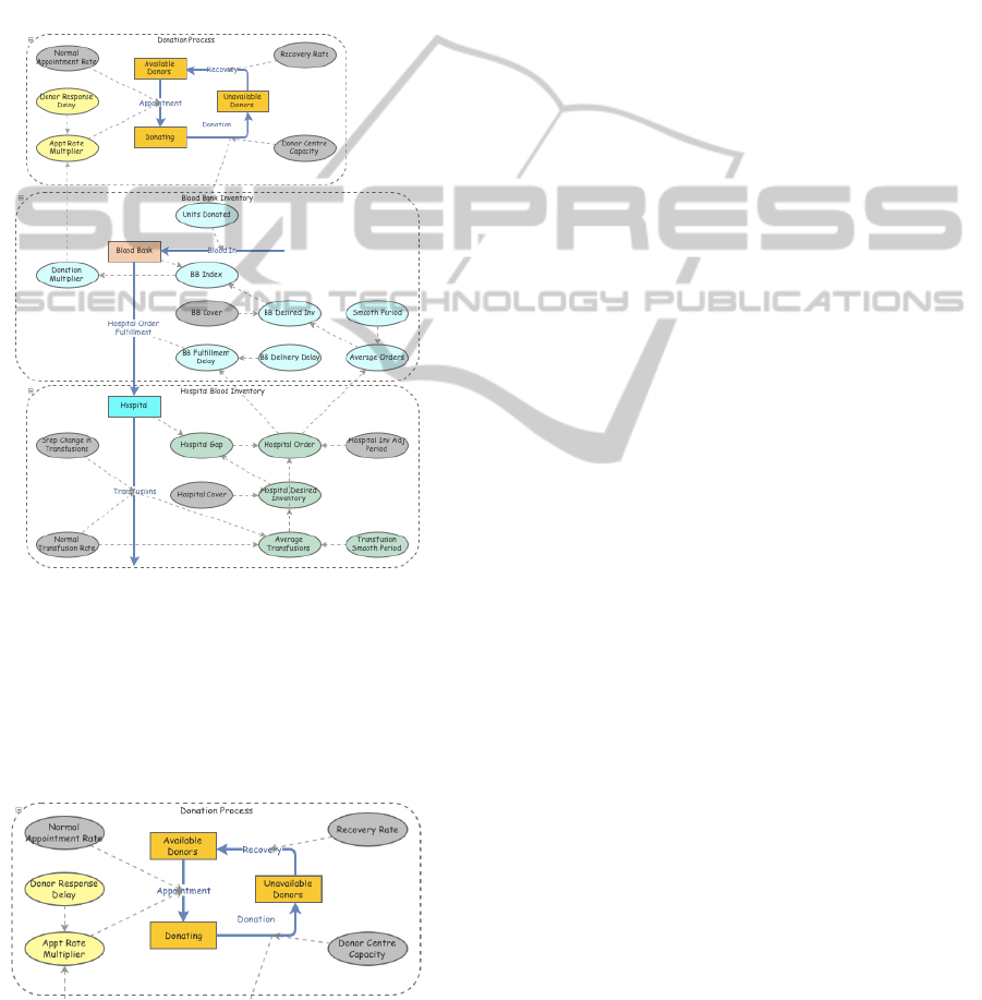
Figure 1: A simple System Dynamics model of a blood in-
ventory built in Insight Maker.
Before we consider the behaviour of the whole
system we consider just the top section of the model
shown below in figure 2 which is concerned with the
donor base. This section will be also be used to de-
scribe the meaning of the various components.
Figure 2: The donor population model in Insight Maker.
Donors move between three states. These are rep-
resented by the three orange rectangular boxes. In
system dynamics parlance these are termed stocks.
A donor will either be available for donation, have
made an appointment to donate or has already do-
nated and is in an 84 day long recovery period. An
available donor will make an appointment to donate
blood. This will cause them to flow along the blue ar-
row from the available donor stock to to the donating
stock. Once blood is taken this donor will then flow
along the blue arrow into the unavailable donors stock
where he will remain for 84 days before recovering
and flowing back into the available state. The quan-
tity of 84 days is analogous to the parameter k given in
section 5.1 above. At the beginning of the simulation
this donor population is divided so that 6 donors are
in the process of donating blood, 504 are available to
give blood and 504 have given blood in the previous
84 days so they are unavailable. The sum of these val-
ues analogous to N
t
. The number of available donors
is analogous to A
t
, the number donating is analagous
to P
t−1
and the number of unavailable donors is anal-
ogous to V
t
· 1
|
k
.
It is no coincidence that these initial values have
been chosen. Since the recovery rate and the normal
appointment rate (represented by pale grey ovals) are
both set at 1/84 the system will remain in equilibrium
with the integer values of the stocks preserved. When
the appointment rate differs from the recovery rate the
system will attempt to converge on a new equilibrium
which is likely to be non-integer valued. In reality
donors are not divisible, but this has been set up to
demonstrate the system behaviour rather than repre-
sent it accurately. Given this motivation, non-integer
values of donors are acceptable.
The pale yellow ovals capture two important prop-
erties of the donation process. The oval marked ‘Appt
Rate Multiplier’ can vary in response to requests from
the blood bank for more or less donations. Such re-
quests are not addressed immediately by the donor
base. Donors take time to respond. The pale yellow
oval marked ‘Donor Response Delay’ captures the ex-
tent of this delay.
Dotted arrows show the direction of influence in
the model. For example, the normal appointment rate
is a factor which determines the number of available
donors which make an appointment. The dotted rect-
angle which surrounds the donation process allows
it to be treated as a single object when building the
model. It has no bearing on the outcome.
The appointment rate multiplier allows the actual
appointment rate to be responsive to the request for
donations made by the blood bank. If we were to as-
sume that there was a request to double the amount of
blood needed for a period of 30 days it can be seen
that the system attempts to reach a new equilibrium
to meet the increased requirement and attempts to re-
ICORES2015-DoctoralConsortium
6
vert to the original level when the requirement ceases.
Convergence to a new equilibrium does not happen
straight away. If the actual appointment rate is chang-
ing constantly in response ot blood bank requirements
the system cannot settle into an equilibrium state.
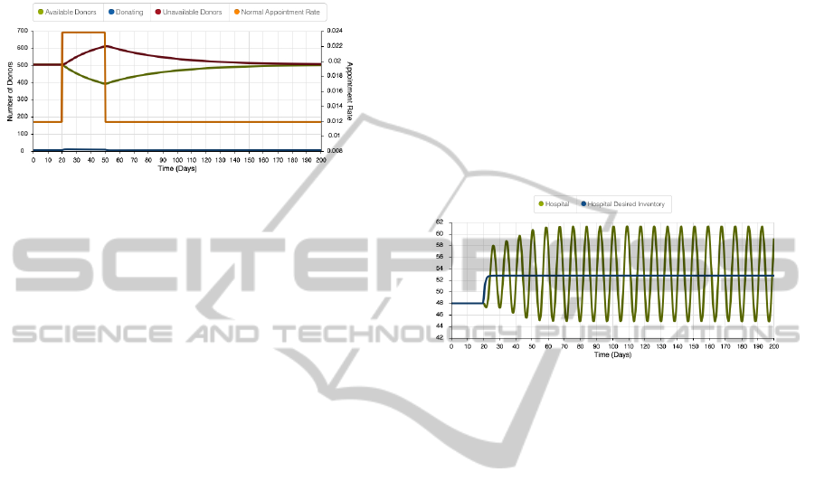
Figure 3: The response of the donor model to a doubling
of the appointment rate for a period of 30 simulation days.
The orange line is plotted using the second Y-axis and rep-
resents a doubling of the appointment rate for a period of
30 days. The green line shows how the number of avail-
able donors falls when the request for additional donations
is made and how it then rises once the request returns to
the initial level. The purple line also shows the comple-
ment of this in the number of unavailable donors. The blue
line shows the number of donors that have made an appoint-
ment.
The use of the three donor states give this model
some similarities to the mathematical framework dis-
cussed earlier. The transition of unavailable donors
to available donors does not account for this in quite
the same way, but it does capture the salient features.
Similar simplifications are present elsewhere in the
model as the intent is to give insight into the behaviour
of the system rather than simulate it exactly.
Now we consider the behaviour of the entire sys-
tem in response to a very small change in transfusions.
The system is in equilibrium until simulation day 20,
at which point the transfusion rate increases by just
10%. Eventually this small increase will cause the
hospital to re-evaluate its desired inventory level. In
turn this will increase the size of the order the hospital
places with the blood bank. In the Australian system,
a hospital may place an order in the morning and re-
ceive it from the blood bank in the afternoon of the
same day. However, there is a larger, notional period
of time between the recognition of a new order level
and when the order is finally made available within its
inventory. In the example we use here this has been
set to 2 days.
When the blood bank starts to notice orders of a
higher level being made it will re-evaluate its desired
inventory level and request additional donations to
meet the increased demand. Donors cannot respond
instantly to the blood bank’s request. They take time
to respond to the request, but ultimately more donors
will make an appointment to give blood. In this exam-
ple we have assumed that it takes 7 days for donors to
respond to a request for more blood. If the number of
appointments exceeds the capacity of the donor centre
surplus donors are moved into the next day. This al-
lows the number of donors with appointment to back-
log should they exceed the capacity of the donor cen-
tre.
Figures 4 to 7 show how these two delays cause
the system to become unstable. The hospital is able
to adjust its desired inventory level quite quickly to
the new requirement. However figure 4 shows that
the actual quantity of blood stored in the hospital’s
inventory begins to oscillate with a frequency of ap-
proximately 7 days.
Figure 4: Response of the hospital inventory to a small in-
crease in transfusion rate. The blue line is the hospital’s
desired inventory level. This moves up solely in response
to the increased level of transfusion. The green line shows
how the actual inventory held in the hospital begins to os-
cillate in response to the increased demand level.
In figure 5 we see that the desired blood bank in-
ventory also begins to oscillate in sympathy with the
hospital inventory. This is because the desired inven-
tory level of the blood bank is driven by the orders
being placed by the hospital. In order to respond to
this the blood bank requests a change in the number
of donations being made. These new donations do not
appear in the system straight away. The actual inven-
tory held by the blood bank becomes quite erratic but
does eventually settle into more consistent oscillatory
behaviour.
The request for additional blood results in more
donors making an appointment. The number of ap-
pointments that can be dealt with though is limited
by the capacity of the donor centre. In figure 6 we
see that this initial increase in donations increases the
number of donors that are unavailable resulting in a
subsequent decrease in donations as the number avail-
able to donate falls. This causes some initial insta-
bility in the donor population which does eventually
settle down but continues to have some small oscilla-
tions.
Oscillations also appear in the units of blood that
are used to fulfil hospital orders. That is because the
order quantities themselves are oscillating. However,
EnsuringBloodisAvailableWhenitisNeededMost
7

Figure 5: Response of the blood bank inventory to a small
increase in the transfusion rate. The green line shows an
oscillation in the blood bank’s desired inventory level. This
is sympathetic to hospital orders for blood. The actual in-
ventory level held by the blood bank, shown by the blue
line, becomes erratic as it is now subject to both the delay
present in the hospital inventory system and the delay in the
response of donors to requests for more blood.
Figure 6: Response of the donor population to a small in-
crease in the number of transfusions. The blue line de-
scribes the number of donors that are waiting to give blood
after having made and appointment. The green line is the
number of donors that are available to make appointments
and the purple line is the number of unavailable donors.
we see in figure 7 that the compounding effect of os-
cillation and delays causes the number of units do-
nated to behave quite erratically. It is also apparent
that the quantity of units donated is limited by the ca-
pacity of the donor centre as we see a plateau from
simulation day 25 to simulation day 40. During this
time appointments were backlogging in the donating
stock.
Figure 7: The number of donations made and the number
of units of blood supplied in fulfilment of hospital orders.
The green line represents hospital orders being fulfilled by
the blood bank. This oscillates in sympathy with hospital
orders but incorporate a delay of 2 days. The blue line is
the number of units of blood donated. This is quite erratic
and has plateaus where the number of appointments exceed
the capacity of the donor centre.
This simple model exhibits behaviour that is
volatile without the need to introduce any stochastic
variables at all. This is consistent with the hypoth-
esis stated in section 3. The potential remains to add
stochastic variables to the model, but leaving them out
gives great insight into the system dynamics making
it difficult to ignore in any mathematical framework
for blood inventories.
5.3 Approach
It is hoped that the simple model shown in the previ-
ous section demonstrates the behaviour that a blood
inventory system is capable of as a result of a very
small change in the number of units of blood trans-
fused. In reality both transfusions of blood and dona-
tions made are stochastic and this has motivated re-
searchers to consider approaches based on stochastic
processes to model the behaviour of these inventories.
However, current and past research has not consid-
ered that a system dynamics view might explain why
real blood inventories exhibit more volatility than that
seen in simulations. This volatility arises because of
delays in the feedback loops inherent the blood inven-
tory system. There are delays when a hospital makes
an order and when that order arrives from the blood
bank. There are delays when the blood bank requests
additional donations. These delays interact with each
other to produce oscillation and instability.
As an analogy, consider what would happen if
there was a material delay between when you turn the
steering wheel of your car and when the car actually
started to turn. The delayed response of the vehicle
and the subsequent feedback you get as you look at
the road ahead would lead to a never ending process
of correction and overcorrection. This is what appears
to be happening with blood inventories. Incorporation
of system dynamics concepts into the mathematical
framework of blood inventories will allow this gap to
be addressed as it is both the stochastic nature of sup-
ply and demand and the structure of the blood inven-
tory system which interact to cause greater volatility
than would otherwise be expected.
6 EXPECTED OUTCOME
Building a model of blood inventories that can cap-
ture realistic dynamics of the blood inventory system
will engender improvements in the management of
blood inventories. Further, it will inform policy mak-
ers as to effective strategies to ensure that shortages
and outdates of blood are minimised. Better models
ICORES2015-DoctoralConsortium
8

will help to ensure that blood is available when it is
needed most.
REFERENCES
Abbasi, B. and Seidmann, A. (2014). Reducing the shelf
life of perishable items with stochastic replenishment
in a two-echelon inventory system. Technical report,
Simon School Working Paper No. FR 14-08.
Abouee-Mehrizi, H., Baron, O., Berman, O., and
Sarhangian, V. (2014). Allocation policies in blood
transfusion. Working Paper.
Arrow, K. J., Harris, T., and Marschak, J. (1951). Optimal
inventory policy. Econometrica, 19(3):250–272.
Atkinson, M., Fontaine, M., Goodnough, L., and Wein, L.
(2012). A novel allocation strategy for blood trans-
fusions: Investigating the tradeoff between the age
and availability of transfused blood. Transfusion,
52(1):108–117.
Blake, J. T. and Hardy, M. (2014). A generic modelling
framework to evaluate network blood management
policies: The canadian blood services experience. Op-
erations Research for Health Care, 3(3):116–128.
Derman, C. and Klein, M. (1958). Inventory depletion man-
agement. Management Science, 4(4):450–456.
Elston, R. C. and Pickrel, J. C. (1963). A statistical ap-
proach to ordering and usage policies for a hospital
blood bank*. Transfusion, 3(1):41–47.
Fortmann-Roe, S. (2014). Insight maker: A general-
purpose tool for web-based modeling & simulation.
Simulation Modelling Practice and Theory, 47(0):28–
45.
Fries, B. E. (1975). Optimal order policy for a perishable
commodity with fixed lifetime. Operations Research,
23:46–61.
Goh, C.-H., Greenberg, B., and Matsuo, H. (1993). Per-
ishable inventory systems with batch demand and ar-
rivals. Operations Research Letters, 13(1):1–8.
Harris, F. W. (1990 [Reprinted from 1913]). How
many parts to make at once. Operations Research,
38(6):947–950.
Millard, D. W. (1959). Industrial inventory models as ap-
plied to the problem of inventorying whole blood.
Nahmias, S. (1975). Optimal ordering policies for per-
ishable inventory-ii.Operations Research, 23(4):735–
749.
Pierskalla, W. P. and Roach, C. D. (1972). Optimal issuing
policies for perishable inventory. Management Sci-
ence, 18(11):603–614.
Prastacos, G. P. (1984). Blood inventory management: An
overview of theory and practice. Management Sci-
ence, 30(7):777–800.
Scarf, H. (1960). The optimality of (s, S) policies in the
dynamic inventory problem. In KJ Arrow, S. Karlin,
P. S., editor, Mathematical Methods in the Social Sci-
ence. Stanford University Press, Stanford.
EnsuringBloodisAvailableWhenitisNeededMost
9
