
A Unified Framework for Coarse-to-Fine Recognition of Traffic Signs
using Bayesian Network and Visual Attributes
Hamed Habibi Aghdam, Elnaz Jahani Heravi and Domenec Puig
Department of Computer Engineering and Mathematics, University Rovira i Virgili, Tarragona, Spain
Keywords:
Traffic Sign Recognition, Visual Attributes, Bayesian Network, Most Probable Explanation, Sparse Coding.
Abstract:
Recently, impressive results have been reported for recognizing the traffic signs. Yet, they are still far from the
real-world applications. To the best of our knowledge, all methods in the literature have focused on numerical
results rather than applicability. First, they are not able to deal with novel inputs such as the false-positive
results of the detection module. In other words, if the input of these methods is a non-traffic sign image, they
will classify it into one of the traffic sign classes. Second, adding a new sign to the system requires retraining
the whole system. In this paper, we propose a coarse-to-fine method using visual attributes that is easily
scalable and, importantly, it is able to detect the novel inputs and transfer its knowledge to the newly observed
sample. To correct the misclassified attributes, we build a Bayesian network considering the dependency
between the attributes and find their most probable explanation using the observations. Experimental results
on the benchmark dataset indicates that our method is able to outperform the state-of-art methods and it also
possesses three important properties of novelty detection, scalability and providing semantic information.
1 INTRODUCTION
Traffic sign detection and recognition is one of the
major tasks in advanced driver assistant systems and
intelligent cars. A traffic sign detection and recogni-
tion system is composed of two modules namely de-
tection and recognition. The input of the detection
module is the image of the scene and its output is the
areas of the image that include a traffic sign. Then,
the recognition module analyses the images of these
areas and recognizes the type of the traffic sign.
One of the important characteristics of traffic signs
is their design simplicity which facilitates their detec-
tion and recognition for a human driver. First, they
have a simple geometric shape such as circle, triangle,
polygon or rectangle. Second, they are distinguish-
able from most of the objects in the scene using their
color. To be more specific, traffic signs are usually
composed of some basic colors such as red, green,
blue, black, white and yellow. Finally, the meaning of
the traffic sign is acquired using the pictograph in the
center. Even though the design is clear and discrim-
inative for a human, but there are challenging prob-
lems in real world applications such as shadow, cam-
era distance, weather condition, perspective and age
of the sign that need to be addressed in the traffic sign
detection and recognition systems.
Moreover, there are two difficulties that must be
tackled by the recognition module in the real-world
applications. First, the traffic sign recognition is a
multi-category classification problem that can include
hundreds of classes. Second, assuming the fact that it
is probable to have some false-positive outputs in the
detection module, the recognition module must dis-
card these false-positive inputs. In other words, the
recognition module must deal with the novel inputs
that have not been observed during the training.
To the best of our knowledge, most of the works in
the recognition module have only focused on increas-
ing the performance of the system under more real-
istic conditions and on a limited number of classes.
Further, none of the methods in the literature have
been tried to recognize the traffic signs in a coarse-to-
fine fashion. Despite the impressive results obtained
by different groups in the German traffic sign bench-
mark competition (Stallkamp et al., 2012), all of these
methods suffer from some common problems.
First, none of the methods in the literature are able
to deal with novel inputs. For example, given the im-
age of a non-traffic sign object (e.g. false-positive re-
sults of the detection module), the state-of-art meth-
ods classify the novel input into one of the traffic sing
classes. Second, they are not easily scalable. On the
one hand, adding a new class to the recognition mod-
87
Habibi Aghdam H., Jahani Heravi E. and Puig D..
A Unified Framework for Coarse-to-Fine Recognition of Traffic Signs using Bayesian Network and Visual Attributes.
DOI: 10.5220/0005303500870096
In Proceedings of the 10th International Conference on Computer Vision Theory and Applications (VISAPP-2015), pages 87-96
ISBN: 978-989-758-090-1
Copyright
c
2015 SCITEPRESS (Science and Technology Publications, Lda.)

ule might require to re-train the whole system. On
the other hand, they use the conventional classifica-
tion method in which we consider that all classes are
well separated in the same feature space and, using
this assumption, a single model is trained for whole
classes. While this assumption can be true for a few
number of classes but it is probable that there will be
an overlap between classes if the number of classes
increases. Third, they do not take into account the
attributes of the traffic signs.
Attributes are high level concepts which provide
some useful information about the objects. For ex-
ample, if we observe that the input image “has red
margin” and “is triangle” and its pictograph depicts
an object that “is pointing to the left” with a high
probability the input image is a “dangerous curve to
the right” traffic sign. In this case, we could rec-
ognize the traffic sign using three attributes. As the
second example, assume the attributes “has red rim”,
“is circle” and “contains a two-digit number” have
been observed. These attributes reveal that the in-
put image indicates a “speed limit” traffic sign. Con-
sidering that there are at most 10 speed limit traffic
signs, we only need to do a 10-class classification in-
stead of hundreds-class classification
1
if we observe
the mentioned attributes before the final classification.
In sum, we believe a successful and applicable traffic
sign recognizer must have the following characteris-
tics: 1) The cost of adding a new class to the system
should be low (scalability). 2) Novel inputs must be
rejected and 3) it should follow a coarse-to-fine clas-
sification approach.
In this paper, we propose a coarse-to-fine method
for recognizing the large number of traffic signs with
ability to identify the novel inputs. In addition, adding
a new class to the system requires to update a few
models instead of the whole system. It should be
noted that our goal is not to notably improve the nu-
merical results of the state-of-art methods since the
current performance is 99% but to propose a more
scalable and applicable method with better perfor-
mance which is also able to detect the novel inputs
and provide some high level information about the
any inputs. To achieve this goal, we first do a coarse
classification on the input image using semantic vi-
sual attributes and classify it into one of the possi-
ble object categories. Then, a fine-grained classifica-
tion is done on the objects of the detected category.
However, because the attributes of the object are de-
tected using a one-versus-all classifier, it is possible
that some attributes of the object are not detected and
some irrelevant attributes are detected for the same
1
we consider that there are at most 100 traffic signs to
be recognized.
object. To deal with this problem, we take into ac-
count the correlation between the different attributes
as well as the uncertainty in the observations and build
a Bayesian network. Next, we enter our observation
to the Bayesian network and select the most proba-
ble explanation of the attributes. Finally, the refined
attributes are used to find the category of the traffic
sign or ascertain if it is a novel input.
Contribution: one of the important aspects of the
proposed method is that all objects in the same cate-
gory share the same attributes. For example, all speed
limit traffic signs are triangle, have a red rim and con-
tain a two-digit or three-digit number. In our pro-
posed method, the input image is in the category of
the speed limit traffic signs if it possesses all these
three attributes. Otherwise, it does not belong to this
category. Using this property, we are able to iden-
tify the novel inputs. More precisely, if the input im-
age does not belong to any of the coarse categories,
it is classified as a novel input. Our second contri-
bution is proposing a scalable method. This means
that the proposed framework can be effectively ex-
tended to hundreds of classes. Our third contribution
is dividing the hundreds of classes into fewer cate-
gories and building separate fine-grained classifiers
for every category. For instance, the category “speed
limit” may contain 10 classes including 8 signs with
different two-digit numbers and 2 signs with differ-
ent three-digit numbers. Clearly, there are subtle dif-
ferences between these signs. For example, the traf-
fic sign “speed limit: 70Km/h” is visually very sim-
ilar to the “speed limit: 20Km/h” sign. As a result,
the classification approach must take into account the
subtle differences rather than more abstract charac-
teristics. Another advantage of dividing the problem
into smaller problems is that in the case of adding a
new sign to the system, we need to find its relevant
category and update only the classification model of
this category. Last but not the least, in the case that
our system cannot find the category of the object or it
is not confident about the classification result, it pro-
vides a more abstract semantic information which can
be fused with the context and temporal information
for inference.
The rest of this paper is organized as follows: Sec-
tion 2 reviews the state-of-art methods for recognizing
the traffic signs as well as the methods for detecting
the attribute of the object. Then, the proposed method
is described in section 3 where we mention the feature
extraction method and the Bayesian network model.
Next, we show the experimental results in section 4
and finally, the paper concludes in section 5.
VISAPP2015-InternationalConferenceonComputerVisionTheoryandApplications
88

2 RELATED WORK
Traffic sign recognition has been extensively studied
and some impressive results on uncontrolled environ-
ments have been reported. In general, the methods for
recognizing the traffic signs can be divided into three
different categories namely template matching, clas-
sification and deep networks.
Template Matching: In the early works, a traffic
sign is considered as a rigid and well-defined object
and their image are stored in the database. Then, the
new input image is compared with the all templates in
the database to find the best matching. The methods
based on template matching usually differ in terms of
similarity measure or template selection. Obviously,
these methods are not stable and accurate in uncon-
trolled environments. For more detail the reader can
refer to (Piccioli et al., 1996) and (Paclik et al., 2006).
Classification: Recently, classification ap-
proaches have achieved high accurate results on
more realistic databases. These approaches consist
of two major stages. In the first stage, features of
the image are extracted and, then, they are classified
using machine learning approaches. Stallkamp et.
al. (Stallkamp et al., 2012) achieved 95% classifi-
cation accuracy on German traffic sign benchmark
database (Houben et al., 2013) by extracting the HOG
features and classifying the images into 43 classes
using the linear discriminant analysis. Zaklouta and
Stanciulescu (Zaklouta and Stanciulescu, 2011)- (Za-
klouta and Stanciulescu, 2014) extracted the same
HOG features on the same database in (Stallkamp
et al., 2012) and classified them using the random
forest model. They could increase the performance
up to 97.2%. Similarly, Sun et. al. (Sun et al.,
2014) utilized extreme learning machine method
for classification of the HOG features and achieved
97.19% accuracy on the same database.
In another study, Maldonado et. al. (Maldonado-
Bascon et al., 2007) (Bascn et al., 2010) recognized
the traffic signs by recognizing the pictographs using
support vector machine. Most recently, Liu et. al.
(Liu et al., 2014) extracted the SIFT features of the
image after transforming it to the log-polar coordi-
nate system and found the visual words using k-means
clustering. Then, the feature vectors were obtained
using a novel sparse coding method and, finally, the
traffic signs were recognized using support vector ma-
chines.
Different from the previous approaches, Wang et.
al. (Wang et al., 2013) employed a two step classi-
fication. In the first step, the input image is classified
into 5 super-classes using HOG features and support
vector machine. In the second stage, the final clas-
sification is done using HOG and support vector ma-
chine after doing perspective adjustment on the image
taking into account the information from the super
class. For more detailed information about classifi-
cation based methods the reader can refer to (Mogel-
mose et al., 2012).
Deep Network: deep networks outperformed the
human performance by classifying more than 99%
of the images, correctly. Ciresan et. al. (Cirean
et al., 2012) (Ciresan et al., 2011) developed a bank of
7-layer deep networks whose inputs are transformed
version of the input image. In addition, Sermanet and
LeCun (Sermanet and LeCun, 2011) proposed a 7-
layer deep network for recognizing the traffic signs
and obtained 99% accuracy in their experiments.
Discussion: Despite the impressive results
achieved by both deep networks and classification
methods, but they are still far from the real applica-
tions. First, a deep network is slow and it cannot
currently be used in real-time applications. Second,
finding the optimal structure of the deep network is a
time consuming task which depends on the number of
the classes. In the other words, if the number of the
classes changes, the whole network need to be trained
again. Third, neither deep network nor the above clas-
sification methods are not able to deal with the novel
inputs and they will classify every input image into
one of the traffic sign classes. To address all these
problems, in this paper, we have formulated the traffic
sign recognition problem in terms of visual attributes
and fine-grained classification.
Visual attributes was first proposed by Ferrari
and Zisserman (Ferrari and Zisserman, 2007) and,
later, it has been successfully used for defining the
objects (Russakovsky and Fei-Fei, 2012). Cheng
and Tan (Cheng and Tan, 2014) classified the flow-
ers by learning attributes using sparse representation.
Farhadi et. al. (Farhadi et al., 2009) described the
objects using semantic and discriminative attributes.
Semantic attributes are more comprehensive and they
are the ones which human use to describe the objects.
They can include shape, material and parts. In con-
trast, discriminative attributes are the ones that does
not have a specific meaning for human but they are
utilized for better separating the objects. One impor-
tant advantage of visual attributes is their ability to
transfer the knowledge to the new classes of objects
and learn them without examples. This is called zero
shot learning and it is illustrated in fig.1. Here, 7 dif-
ferent attributes are learned and they can be identified
in the input images. As it is shown in this figure, by
detecting the correct attributes of the input image we
are able to recognize 11 signs without observing them
during the training phase. This is an important prop-
AUnifiedFrameworkforCoarse-to-FineRecognitionofTrafficSignsusingBayesianNetworkandVisualAttributes
89

Figure 1: Zero-shot learning using a set of attributes.
erty which can help us to extend our models with a
few efforts through transferring the knowledge from
observed classes to the new classes (Rohrbach et al.,
2010) (Lampert et al., 2009).
3 PROPOSED METHOD
Traffic sign recognition is a multi-category classifi-
cation problem with hundreds of classes. Also, it is
not trivial to collect a large number of real-world im-
ages of every sign. Further, some signs happens more
frequently than other signs. For example, it is more
probable to see the “curve” signs instead of the “be
ware of snow” sign. For this reason, the collected
database might be highly unbalanced. Consequently,
the trained model for the signs with fewer data can be
less accurate than the ones with more data. One fea-
sible remedy to this problem is to update the models
through time. However, if we build a single model for
classification of all signs, it will be a time consuming
task to re-train this model. But, if we can group the
N traffic signs into M < N categories
2
, then, we can
train a different model for each category and in the
case of adding new signs, we need to find its relevant
category and re-train only the model of this category.
On the other hand, temporal information plays an
important role in human inference system. For ex-
ample, if we observe “no passing” sign at time t
1
we
expect to see “end of no passing zone”, after a while,
at time t
2
. Assume the sign “end of no passing zone”
is impaired because of its age and it is hard to see its
pictograph and the stripped crossing. In this case, if
we follow the classification approaches that we men-
tioned in the previous section, the “end of no passing
zone” sign can be incorrectly classified. However, if
we provide some more abstract information such as
“the input image has a circular shape and black-white
color,” the traffic sign recognition system can infer
that the image is related to the previously observed
“no passing” sign. Hence, it probably indicates the
“end of no passing zone” traffic sign.
In this paper, we propose a coarse-to-fine classifi-
cation approach using the semantic attributes of the
2
A category may contain more than one traffic sign.
object. Fig.2 shows the overview of the proposed
algorithm. In the first stage, the image is divided
into several regions and each region is coded using a
sparse coding method. Then, the feature vector is ob-
tained by concatenating the locally pooled coded vec-
tors (Section 3.1). Next, the feature vector is individ-
ually applied on the attribute classifiers and the clas-
sification score of each attribute is computed (Sec-
tion 3.2). Finally, the certain state of each attribute
is estimated by plugging the scores into the Bayesian
network and calculating the most probable explana-
tion of the attributes (Section 3.3). In the next step,
the category of the image is found using the attribute
configuration (Section 3.4). Having the sign category
found, the fine-grained classifier of this category is
used to do the final classification (Section 3.5).
3.1 Feature Extraction
In order to train the attribute classifiers, we first need
to extract the features of the traffic sign. The extracted
feature must be able to encode the color, the shape and
the content of the traffic sign in the same vector. One
of the characteristics of the traffic sign is that they are
rigid and their geometrical features ( e.g. shape, size
and orientation) as well as their appearance (e.g. color
and content) remains relatively unchanged. From this
point of view, a simple template matching approach
can be useful for the recognition task. However, some
important issues such as motion blur, weather condi-
tion and occlusion cause the template matching ap-
proach to fail.
Nonetheless, it is possible to divide the image of
the traffic signs into smaller blocks and learn the most
dominant exemplars of each block, independently.
Then, we can reconstruct the original block by lin-
early combining the exemplars. This is the idea be-
hind sparse coding approach (Lee et al., 2007). More
specifically, as it is shown in fig.3, we divide the in-
put image into 5 different regions and each region is
divided into a few smaller blocks. For example, the
region indicated by number 1 is divided into 3 blocks.
Then, in order to learn the templates of the region r,
we first collect the images of the blocks of this re-
gion from all training images and, then, learn the most
dominant exemplars by solving the following equa-
tion:
minimize
D
r
, α
r
1
n
∑
n
i=1
1
2
kx
r
i
− D
r
α
r
i
k
2
2
sub ject to kα
r
i
k
1
<= λ
(1)
In this equation, x
r
i
∈ R
M
is a M-dimensional vector
representing the RGB values of the blocks in region
r, D
r
is a R
M×K
matrix storing the K dominant tem-
plates of region r in the training images, α
r
i
∈ R
K
is a
VISAPP2015-InternationalConferenceonComputerVisionTheoryandApplications
90
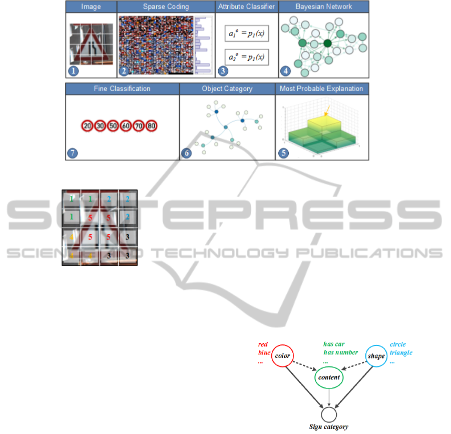
Figure 2: Overview of the proposed method (best viewed in color).
Figure 3: Feature extraction scheme.
K-dimensional sparse vector indicating the templates
which have been selected to reconstruct the block x
r
i
and λ is the value which controls the sparsity. The
value of λ is determined empirically by the user.
After training the dictionaries, we can use them to
extract the features of the input images. To this end,
we divide the input image into regions and blocks in
the same way that it is shown in fig.3. Then, we take
the blocks of each region r, separately, and minimize
(1) assuming that the values of D are fixed in order
to compute the vector α
r
i
of each block. At this step,
we have a few K-dimensional vectors. For example,
we will obtain four vectors from region 5. Then, the
feature vector of region r is computed by pooling the
vectors in that region:
f
r
=
n
r
∑
i=1
α
r
i
(2)
In this equation, n
r
is the number of the blocks in re-
gion r. Finally, the feature vector of the image is ob-
tained by concatenating the vectors f
r
, r = 1 . . . 5 into
a single vector and normalizing it using L
1
norm.
3.2 Attribute Classifier
A traffic sign can be defined using three sets of visual
attributes. These are illustrated in fig.4. Dashed
arrows show the soft dependency relation and we
will discuss about them in the next section. In
fact, there is a causal relationship between these
attributes and the traffic signs. In the other words, we
can verify the validity of this relationship using the
concept of ancestral sampling. Given the color, shape
and content attributes, we can randomly generate
new traffic signs using the probability distribution
function p(tra f f ic sign|color, shape, content). For
instance, while p(tra f f ic sign = curve le f t|color =
red, shape = circle, content = has number)
might be close to zero but p(tra f f ic sign =
speed limit 60|color = red, shape = circle, content =
has number) is high.
Figure 4: Causal relationship between the attributes and the
traffic signs.
Taking this causal relationship into account, we
have defined three sets of attributes including color
(4 attributes), shape (3 attributes) and content (12 at-
tributes). These attributes are listed in table 1. Each
traffic sign in our experiments can be described using
these attributes. However, they can be easily extended
to more attributes without affecting the general model
we have proposed in this paper.
Detecting the attributes of the input image is done
through the attribute classifiers. For this reason, we
need to train 19 binary classifiers as follows. For each
attribute, we select the images having that attribute
as the positive samples and the rest of the images as
the negative samples. Then, we train a random forest
AUnifiedFrameworkforCoarse-to-FineRecognitionofTrafficSignsusingBayesianNetworkandVisualAttributes
91

Table 1: Sets of attributes for describing the traffic signs.
Content
has human(a
1
) danger road(a
2
) pointing up(a
3
)
end of (a
4
) 2-digit number(a
5
) pointing right(a
6
)
has car(a
7
) 3-digit number(a
8
) pointing left(a
9
)
has truck(a
1
0) irregular object(a
1
1) is blank(a
1
2)
Color
red(a
1
3) blue(a
1
4) yellow(a
1
5)
black-white(a
1
6)
Shape
circle(a
1
7) triangle(a
1
8) polygon(a
1
9)
model on the collected data. At the end, we will have
19 random forest models for finding the attributes of
the input image.
3.3 Bayesian Network Model
Fig.5 shows the general model for the classification
of the images using attributes where x indicates the
feature vector, a
i
, i = 1 . . . N is a binary value indicat-
ing the presence or absence of the i
th
attribute and
y
k
, k = 1 . . . K is the class label.
Figure 5: General classification model using attributes.
Based on this model, it is easy to show that the
classification will be done by finding the maximum a
posteriori of the class labels:
y
∗
= arg max
k=1...K
∑
a=0,1
p(a|x)p(y
k
|a) (3)
where a = a
i
|i = 1 . . . N is a binary vector. There are
two important issues with this model. First, it does
not take into account the causal relationship between
the attributes and it considers them completely inde-
pendent. This means, using this model, the attribute
“danger in road ” does not longer depend on the shape
attributes. But, all traffic signs indicating the danger
will be only shown in the red and triangle signs. Sup-
pose that we observe the attributes “is blue ”, “is tri-
angle ” and “pointing left”. Obviously, there is no
traffic sign with this configuration. However, if the
shape had been detected as “is circle “or the color had
been detected as “is red”, the configuration was valid.
But, with the model of fig.5 it is difficult to find which
attribute has been falsely classified. The reason is it
does not take into account the dependency between at-
tributes and the uncertainty of the observations. The
second issue is that ,using this model, detecting the
novel inputs is not a trivial task. In order to detect the
novel inputs, we need to define a threshold which can
be compared with the maximum a posteriori value for
this purpose. However, determining the value of the
threshold is an empirical task and it highly depends on
the conditional distribution models of each attribute.
On the other hand, if one of the models changes, we
need to find the threshold value, again.
As we mentioned in fig.4, the image of the traf-
fic sign can be described in terms of color, shape and
content (pictograph). However, there is also a soft
dependency between the content and other attributes
(dashed lines). This is because some attributes can
happen regardless of the shape and color. For exam-
ple, the content attribute “is blank” can happen on ev-
ery possible combination of the color and the shape
attributes. In other words, the attribute “is blank” can
be independent of the other attributes. In addition,
there is also intra-dependency between the content at-
tributes. For example, if we observe “has truck” at-
tribute, it is probable to observe “has car ” attribute,
as well (e.g. “no passing” traffic sign). To find the
dependencies between the all attributes in table 1, we
calculated the co-occurrence matrix of the attributes.
This is illustrated in fig.6.
Figure 6: Co-occurrence matrix of the attributes.
The co-occurrence matrix is a 19 × 19 matrix
where the element (i, j) in this matrix indicates
the probability of observing i
th
and j
th
attributes
at the same time among the whole classes of traf-
fic signs. Using the co-occurrence matrix, we cre-
ate our Bayesian network by discarding the relations
where their probability in the co-occurrence matrix is
less than the threshold T . Fig.7 shows the obtained
Bayesian network.
VISAPP2015-InternationalConferenceonComputerVisionTheoryandApplications
92

Figure 7: Bayesian network without observation nodes.
The nodes in this Bayesian network depicts the
state of an attribute. In other words, all of the nodes in
this network are binary nodes and they represent the
conditional probabilities of the child attributes given
their parents that are acquired using the training data.
Our goal is to find the optimal state of the attributes
using the identified evidences from the image. For
this reason, we add another 19 observation nodes to
the network. This is illustrated in fig.8 where the solid
gray circles are the hidden nodes and the white cir-
cles are the evidence nodes. Our observations are the
scores of the attribute classifiers (random forests) that
is a number between 0 and 100. Given the evidence
from the attribute classifiers, our goal is to maximize
following function:
a
∗
1
. . . a
∗
19
= argmax
a
1
...a
19
∈[0 1]
19
p(a
1
. . . a
19
, O
a
1
. . . O
a
19
) (4)
where O
a
i
, i = 1 . . . 19 is the score of the i
th
attribute
obtained from the i
th
random forest model. According
to the equation, we are looking for the state of the
hidden variables (actual state of the attributes) such
that the joint probability of the hidden variables and
the observed attributes are maximum. This is called
most probable explanation problem.
3.4 Category Finding
Given the set of 19 attributes, we can cluster the traf-
fic signs into smaller categories. To this end, we
manually specify which attributes are active for each
class of traffic signs. For example, only attributes
red, circle, 2-digit number are active on traffic sign
“speed limit 60”. Then, we cluster the classes with
exactly the same active attributes into one category.
We applied this procedure on the German traffic sign
database and reduced the number of classes from 43
classes into 29 categories. Fig.9 shows the statistic of
different categories as well as the traffic signs inside
Figure 8: Bayesian network after adding observation nodes.
each category. As it is clear from the figure, there are
6 categories with more than one traffic sign and other
categories contain only one traffic sign. This means
that 22 traffic signs can be recognized using their vi-
sual attributes and they do not need a finer classifica-
tion. In contrast, the traffic signs inside the other 6
categories can be recognized by the fine classification
models.
Having the optimal state of the attributes esti-
mated using (4), we can find the category of the new
image using the parsing tree illustrated in fig.10. In
this tree, orange nodes are the starting points and the
white nodes are the leaf nodes.
Novelty Detection: One interesting property of
the parsing tree in fig.10 is that we can use it for find-
ing the novel inputs. To achieve this, we start by the
comparing the optimal state of the attributes obtained
from (4) with the starting nodes. For example, assume
the state of the attribute blue is active and state of the
other color attributes are inactive. According to the
parsing tree, there is only one outgoing path from the
node blue that is the circle attribute. If it is active,
then we keep do parsing, otherwise the input is novel
because the node blue is not a leaf node and the pars-
ing is not successful. In sum, an input image is novel
if there is no active path from the starting points to the
leaf nodes.
3.5 Fine Classification
We saw that a few categories contain more than one
traffic sign. If the input image belongs to one of these
categories, then, the actual class of the image is found
using a fine classification model which is trained on
the images of the category. In other words, we cre-
ate an individual model for every object category with
more than one class inside the category. We follow
the same method as in (Zaklouta and Stanciulescu,
AUnifiedFrameworkforCoarse-to-FineRecognitionofTrafficSignsusingBayesianNetworkandVisualAttributes
93
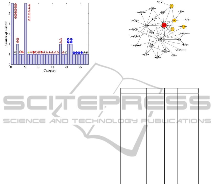
Figure 9: Clustering the traffic signs using visual attributes.
2011) for classifying the objects within the same cat-
egory. Moreover, using our method, we reduce the
number of the classes from 43 to 6 in German traffic
sign benchmark database which is about 7 times re-
duction in the number of classes. Therefore, we only
need to do a 6-class classification instead of 43-class
classification that can be more accurate and flexible.
4 EXPERIMENTS
We have applied our proposed method on the Ger-
man traffic sign benchmark database (Stallkamp et al.,
2012). This database consists of 43 classes. It also in-
cludes two different sets for training and testing. We
have resized the all images into 40 × 40 pixels before
applying any feature extraction method. We have two
sets of feature vectors. The first set which is obtained
by sparse coding method mentioned in this paper is
for recognizing the attributes of the image and the
second set is the HOG features for fine-classification.
For sparse coding approach we applied our proposed
method on both RGB and the distance transform of
the edge image. Then, we concatenated the pooled
vectors to build the final feature vector. For HOG fea-
tures, we utilized the same configuration in (Zaklouta
and Stanciulescu, 2011). Next, we trained two sets of
random forest model one for the attribute classifica-
tion (19 classifiers) and one for the fine classification
of the categories with more than one traffic sign (6
classifiers) using only the training set.
It is worth mentioning that the conditional prob-
abilities of the hidden variables of the Bayesian net-
work are modeled using the conditional probability
tables and the conditional probability of the observa-
tions are modeled using Gaussian distribution of the
attribute scores.
Table 2 shows the results of the attribute classifica-
Figure 10: Parsing tree for finding the category of the im-
age.
Table 2: Precision, Recall and F
1
measure of the attribute
classifiers.
Attribute precision recall F
1
measure
red 0.993 0.990 0.992
blue 0.988 0.992 0.990
yellow 0.971 0.948 0.959
black-white 1.0 0.992 0.996
triangle 0.985 0.995 0.990
circle 0.997 0.987 0.992
polygon 0.991 0.988 0.990
pointing left 0.967 0.947 0.975
pointing right 0.982 0.935 0.957
pointing up 0.994 0.954 0.973
end of 1.0 0.992 0.996
has car 0.993 0.983 0.988
has truck 1.0 0.977 0.988
2-digit number 0.983 0.973 0.978
3-digit number 0.959 0.965 0.962
has human 0.988 0.896 0.940
danger in road 0.932 0.960 0.946
irregular object 0.977 0.913 0.944
is blank 0.991 0.993 0.992
tion on the test dataset. Apparently, the attribute clas-
sifiers have achieved high accuracy in detecting the
attributes of the input images. Next, we tried to find
the category of the test images using the attribute clas-
sification model depicted in fig.5 and our proposed
method. Table 3 and Table 4 show the results of the
category classification using the proposed method and
the general model, respectively. Clearly, our method
has outperformed the general attribute classification
model. The reason is that, using our method, we are
able to model the uncertainties of the observations
and correct the mistakes. Consequently, the number
of the samples that pass the tests in the parsing tree
increases.
In addition, fig.9 reveled that some categories con-
tain only one class. However to compare our results
with other methods, we also applied the fine classi-
fication model on the categories with more than one
class inside. Then, to be consistent with the state-
of-art results, we computed the mean accuracy of the
VISAPP2015-InternationalConferenceonComputerVisionTheoryandApplications
94

Table 3: The result of category classification using the proposed method. The categories are indexed according to fig.9.
Category C
0
C
1
C
2
C
3
C
4
C
5
C
6
C
7
C
8
C
9
C
10
C
11
C
12
C
13
precision 0.998 1.0 0.995 0.993 0.996 0.992 1.0 0.996 0.995 0.993 1.0 0.967 1.0 0.960
recall 0.995 1.0 0.987 1.0 0.996 0.992 1.0 0.998 1.0 1.0 0.980 0.991 0.936 0.941
accuracy 0.994 1.0 0.983 0.993 0.993 0.984 1.0 0.994 0.995 0.993 0.980 0.960 0.936 0.905
Category C
14
C
15
C
16
C
17
C
18
C
19
C
20
C
21
C
22
C
23
C
24
C
25
C
26
C
27
C
28
precision 1.0 0.976 0.985 1.0 0.988 0.961 1.0 0.998 0.992 0.991 0.965 0.965 0.961 1.0 1.0
recall 0.985 0.984 0.987 0.969 0.988 1.0 1.0 0.992 0.977 0.986 0.988 0.965 1.0 1.0 1.0
accuracys 0.985 0.960 0.973 0.969 0.977 0.961 1.0 0.990 0.970 0.978 0.955 0.933 0.961 1.0 1.0
Table 4: The result of category classification using the general model in fig.5. The categories are indexed according to fig.9.
Category C
0
C
1
C
2
C
3
C
4
C
5
C
6
C
7
C
8
C
9
C
10
C
11
C
12
C
13
precision 0.998 1.0 0.981 0.996 1.0 0.972 1.0 0.998 1.0 0.993 1.0 0.725 0.943 1.0
recall 0.958 0.895 0.896 0.972 0.946 0.925 0.899 0.966 0.979 0.979 0.981 0.952 0.688 0.365
accuracy 0.956 0.895 0.881 0.969 0.946 0.901 0.899 0.964 0.979 0.973 0.981 0.699 0.660 0.365
Category C
14
C
15
C
16
C
17
C
18
C
19
C
20
C
21
C
22
C
23
C
24
C
25
C
26
C
27
C
28
precision 1.0 1.0 0.991 1.0 0.929 0.814 1.0 0.996 0.962 0.996 0.977 1.0 0.886 1.0 1.0
recall 0.718 0.944 0.844 0.715 0.824 0.946 0.778 0.930 0.933 0.982 0.977 0.966 0.984 0.840 0.947
accuracy 0.718 0.944 0.838 0.715 0.775 0.778 0.778 0.927 0.899 0.978 0.955 0.966 0.873 0.840 0.947
Table 5: The result of category classification using the proposed method. The categories are indexed according to fig.9.
Speed limits Other prohibitions De-restriction Mandatory Danger Unique
Our method 97.01 99.25 100 97.09 96.31 98.76
Random forests 95.95 99.13 87.50 99.27 92.08 98.73
LDA 95.37 96.80 85.83 97.18 93.73 98.63
classifications. Table 5 shows the results. As it is
clear, there is a significant improvement in recogni-
tion of de-restriction signs (you can refer to (Stal-
lkamp et al., 2012) for definitions of different signs).
This is because the shape of de-restrictions signs is
very similar to some of the signs in other classes. For
example, “end of no-passing” sign has a very simi-
lar edge features to the “no passing” signs. On the
other hand, two other methods represented in this pa-
per have utilized HOG features for classification. Ob-
viously, because of shape similarity of the other signs
with the de-restrictions signs, their feature vector will
be similar, as well. For this reason, there is an over-
lap between the feature vector of this signs with other
signs in the feature space which causes the misclassi-
fication.
However, because our method utilizes the at-
tributes of the image, it is able to model the color,
shape and content of each sign explicitly. For this
reason, when an image from de-restrictions group
is given to our method, it is able to distinguish be-
tween them with other signs simply using the color
attributes. As the result, it is able to improve the ac-
curacy of the classification.
5 CONCLUSION
In this paper, we proposed a method based on visual
attributes and Bayesian network for recognizing the
traffic signs. Our method is different from the state-
of-art methods for various reasons. First, it is more
scalable and in some cases it is possible to learn the
new classes without any training samples (zero-shot
learning). Further, in the case that zero shot learn-
ing is not applicable, the system only requires to up-
date the models locally instead of the whole mod-
els. Second, it is able to detect the novel inputs. In
other words, if there are some false-positive results
in the detection module, our method is able to dis-
card this novel inputs instead of classifying them as
one of the traffic signs. We believe, this is the first
time that novelty detection is introduced for traffic
sign recognition problem. Third, because of using
the visual attributes, our method is able to provide
some high level semantic information about the in-
put image. Fourth, the system is easily expendable
to hundreds of classes of traffic signs since it breaks
the hundred classes to the categories with much less
traffic signs which make them more tractable to clas-
sify without affecting the accuracy of the system. Our
experiments on the German traffic sign benchmark
dataset indicates that in addition to improvements in
the results compared with the state-of-art methods,
AUnifiedFrameworkforCoarse-to-FineRecognitionofTrafficSignsusingBayesianNetworkandVisualAttributes
95

our modeling framework is more closer to the real-
world applications.
REFERENCES
Bascn, S. M., Rodrguez, J. A., Arroyo, S. L., Caballero,
A. F., and Lpez-Ferreras, F. (2010). An optimization
on pictogram identification for the road-sign recogni-
tion task using {SVMs}. Computer Vision and Image
Understanding, 114(3):373 – 383.
Cheng, K. and Tan, X. (2014). Sparse representations based
attribute learning for flower classification. Neurocom-
puting, 145(0):416 – 426.
Cirean, D., Meier, U., Masci, J., and Schmidhuber, J.
(2012). Multi-column deep neural network for traf-
fic sign classification. Neural Networks, 32(0):333 –
338. Selected Papers from {IJCNN} 2011.
Ciresan, D., Meier, U., Masci, J., and Schmidhuber, J.
(2011). A committee of neural networks for traffic
sign classification. In Neural Networks (IJCNN), The
2011 International Joint Conference on, pages 1918–
1921.
Farhadi, A., Endres, I., Hoiem, D., and Forsyth, D. (2009).
Describing objects by their attributes. In Computer
Vision and Pattern Recognition, 2009. CVPR 2009.
IEEE Conference on, pages 1778–1785.
Ferrari, V. and Zisserman, A. (2007). Learning visual at-
tributes. In Advances in Neural Information Process-
ing Systems.
Houben, S., Stallkamp, J., Salmen, J., Schlipsing, M., and
Igel, C. (2013). Detection of traffic signs in real-world
images: The German Traffic Sign Detection Bench-
mark. In International Joint Conference on Neural
Networks, number 1288.
Lampert, C., Nickisch, H., and Harmeling, S. (2009).
Learning to detect unseen object classes by between-
class attribute transfer. In Computer Vision and Pat-
tern Recognition, 2009. CVPR 2009. IEEE Confer-
ence on, pages 951–958.
Lee, H., Battle, A., Raina, R., and Ng, A. Y. (2007). Ef-
ficient sparse coding algorithms. In Sch
¨
olkopf, B.,
Platt, J., and Hoffman, T., editors, Advances in Neural
Information Processing Systems 19, pages 801–808.
MIT Press.
Liu, H., Liu, Y., and Sun, F. (2014). Traffic sign recogni-
tion using group sparse coding. Information Sciences,
266(0):75 – 89.
Maldonado-Bascon, S., Lafuente-Arroyo, S., Gil-Jimenez,
P., Gomez-Moreno, H., and Lopez-Ferreras, F. (2007).
Road-sign detection and recognition based on support
vector machines. Intelligent Transportation Systems,
IEEE Transactions on, 8(2):264–278.
Mogelmose, A., Trivedi, M., and Moeslund, T. (2012).
Vision-based traffic sign detection and analysis for in-
telligent driver assistance systems: Perspectives and
survey. Intelligent Transportation Systems, IEEE
Transactions on, 13(4):1484–1497.
Paclik, P., Novovicova, J., and Duin, R. P. W. (2006).
Building road sign classifiers using trainable similar-
ity measure. IEEE Transactions on Intelligent Trans-
portation Systems, 7(3):309–321. to appear.
Piccioli, G., Micheli, E. D., Parodi, P., and Campani, M.
(1996). A robust method for road sign detection and
recognition.
Rohrbach, M., Stark, M., Szarvas, G., Gurevych, I., and
Schiele, B. (2010). What helps where – and why? se-
mantic relatedness for knowledge transfer. In IEEE
Conference on Computer Vision and Pattern Recogni-
tion (CVPR).
Russakovsky, O. and Fei-Fei, L. (2012). Attribute learning
in large-scale datasets. In Proceedings of the 11th Eu-
ropean Conference on Trends and Topics in Computer
Vision - Volume Part I, ECCV’10, pages 1–14, Berlin,
Heidelberg. Springer-Verlag.
Sermanet, P. and LeCun, Y. (2011). Traffic sign recogni-
tion with multi-scale convolutional networks. In Neu-
ral Networks (IJCNN), The 2011 International Joint
Conference on, pages 2809–2813.
Stallkamp, J., Schlipsing, M., Salmen, J., and Igel, C.
(2012). Man vs. computer: Benchmarking machine
learning algorithms for traffic sign recognition. Neu-
ral Networks, 32(0):323 – 332. Selected Papers from
{IJCNN} 2011.
Sun, Z.-L., Wang, H., Lau, W.-S., Seet, G., and Wang, D.
(2014). Application of bw-elm model on traffic sign
recognition. Neurocomputing, 128(0):153 – 159.
Wang, G., Ren, G., Wu, Z., Zhao, Y., and Jiang, L. (2013).
A hierarchical method for traffic sign classification
with support vector machines. In Neural Networks
(IJCNN), The 2013 International Joint Conference on,
pages 1–6.
Zaklouta, F. and Stanciulescu, B. (2011). Warning traffic
sign recognition using a hog-based k-d tree. In In-
telligent Vehicles Symposium (IV), 2011 IEEE, pages
1019–1024.
Zaklouta, F. and Stanciulescu, B. (2014). Real-time traf-
fic sign recognition in three stages. Robotics and Au-
tonomous Systems, 62(1):16 – 24. New Boundaries of
Robotics.
VISAPP2015-InternationalConferenceonComputerVisionTheoryandApplications
96
