
Improved Automatic Recognition of Engineered Nanoparticles in
Scanning Electron Microscopy Images
Stephen Kockentiedt
1,2
, Klaus Toennies
1
, Erhardt Gierke
2
, Nico Dziurowitz
2
, Carmen Thim
2
and Sabine Plitzko
2
1
Department of Simulation and Graphics, Otto von Guericke University Magdeburg, Magdeburg, Germany
2
Federal Institute for Occupational Safety and Health, Berlin, Germany
Keywords:
Computer Vision, Machine Learning, Nanoparticles, Particle Classification, Scanning Electron Microscopy.
Abstract:
The amount of engineered nanoparticles produced each year has grown for some time and will grow in the
coming years. However, if such particles are inhaled, they can be toxic. Therefore, to ensure the safety of
workers, the nanoparticle concentrations at workplaces have to be measured. This is usually done by gathering
the particles in the ambient air and then taking images using scanning electron microscopy. The particles in
the images are then manually identified and counted. However, this task takes much time. Therefore, we
have developed a system to automatically find and classify particles in these images (Kockentiedt et al., 2012).
In this paper, we present an improved version of the system with two new classification feature types. The
first are Haralick features. The second is a newly developed feature which estimates the counts of electrons
detected by the scanning electron microscopy for each particle. In addition, we have added an algorithm to
automatically choose the classifier type and parameters. This way, no expert is needed when the user wants
to train the system to recognize a previously unknown particle type. The improved system yields much better
results for two types of engineered particles and shows comparable results for a third type.
1 INTRODUCTION
Nanoparticles have diameters between 1 nm and
100 nm and are used in all kinds of products such
as deodorants or sun cream. These are called en-
gineered nanoparticles as they are intentionally pro-
duced rather than being a byproduct of a process such
as combustion. However, in addition to having spe-
cial properties because of their size, they can also be
toxic if they are inhaled (Ostrowski et al., 2009). This
poses a threat to workers producing or handling such
particles. Therefore, there is a need to measure the
concentration of engineered nanoparticles in work en-
vironments.
So-called particles counters can measure the con-
centrations of particles of different sizes in the air.
However, they cannot distinguish between engineered
nanoparticles and other particles, so-called back-
ground particles, such as diesel soot, which is com-
mon in urban environments (Savolainen et al., 2010).
Therefore, particles in the air are gathered using a
so-called precipitator and later, images of them are
taken using a scanning electron microscope (SEM).
By counting the engineered nanoparticles in the im-
ages, their concentration in the sampled air can be es-
timated. This job is typically done by humans. How-
ever, counting the particles is very time-consuming.
Therefore, we have developed a system to automati-
cally detect and classify particles in SEM images to
allow the measurement of the concentration of engi-
neered particles.
In Fig. 1, a few examples of particles in SEM
images can be seen. Fig. 1(a) shows a single engi-
neered nanoparticle made of titanium dioxide (TiO
2
)
with a diameter of about 25 nm. However, much more
common are so-called agglomerates such as the one
in Fig. 1(c), which are multiple nanoparticles stick-
ing together. Both single nanoparticles and agglom-
erates are called particles. If we specifically want to
refer to a single nanoparticle, either as part of an ag-
glomerate or by itself, we will call it primary par-
ticle. Fig. 1 also shows very well how similar en-
gineered nanoparticles of a certain size range are to
background particles such as diesel soot. Figures 1(a)
and 1(b) show primary particles of TiO
2
and diesel
soot, respectively. Apart form differences in contrast,
the images are indistinguishable. Similarly, agglom-
erates are also very similar as can be seen in Figs. 1(c)
337
Kockentiedt S., Tönnies K., Gierke E., Dziurowitz N., Thim C. and Plitzko S..
Improved Automatic Recognition of Engineered Nanoparticles in Scanning Electron Microscopy Images.
DOI: 10.5220/0005299003370344
In Proceedings of the 10th International Conference on Computer Vision Theory and Applications (VISAPP-2015), pages 337-344
ISBN: 978-989-758-090-1
Copyright
c
2015 SCITEPRESS (Science and Technology Publications, Lda.)
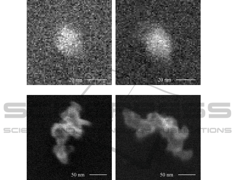
(a) A single TiO
2
primary particle. (b) A single diesel soot primary particle.
(c) A TiO
2
agglomerate. (d) A diesel soot agglomerate.
Figure 1: A comparison of SEM images (1 pixel = 1.27 nm) of TiO
2
nanoparticles with an average diameter of 25 nm on the
left and diesel soot on the right.
and 1(d). This makes it a challenging classification
task because diesel soot is very common in industrial
environments.
We want to find the following nanoparticle types:
• Silver (Ag) with an average diameter of 75 nm.
• Titanium dioxide (TiO
2
) with an average diameter
of 25 nm.
• Zinc oxide (ZnO) with an average diameter of
10 nm.
The SEM images we use for this paper each have a
size of 4000 ×3200. About half of them have a pixel
size of 5.1 nm whereas the other ones have a resolu-
tion of 1.3 nm per pixel. We assume that the software
knows beforehand which type of engineered nanopar-
ticles it has to find and that only this type plus all pos-
sible background particle types can occur. This as-
sumption is realistic as there is usually only one type
of engineered nanoparticles being produced or pro-
cessed at a time.
2 RELATED WORK
To the best of our knowledge, there are only two other
approaches conquering a similar problem on similar
particles (Oleshko et al., 1996; Oster, 2010). How-
ever, there are several differences to our problem.
Oleshko et al. examine similar nanoparticles to
those analyzed by us, but use electron energy loss
spectroscopy instead of SEM. They have access to the
chemical composition of each agglomerate, which we
have not. Apart from that, they only use one feature
called fractal dimension, which only gives a single
number per agglomerate. Additionally, their aim is
to do a characterization of the particles instead of a
classification.
Oster, similar to us, classifies nanomaterials on
VISAPP2015-InternationalConferenceonComputerVisionTheoryandApplications
338

SEM images. However, instead of trying to find engi-
neered nanoparticles, he is searching for carbon nan-
otubes. In addition, being a bachelor’s thesis, his
work was targeted at samples with a limited set of
background particle types, namely diesel soot and
quartz dust.
3 METHOD
The system presented in this paper is an improved ver-
sion of the system we have proposed in (Kockentiedt
et al., 2012). Its workflow has three steps: segmenta-
tion, feature computation and classification. The first
step splits the image into foreground—made up of all
particles—and background. In the second step, for
each connected component of the foreground, several
numerical features are computed. In the classification
step, a classifier uses the feature values to assign each
connected component to either engineered nanoparti-
cles or background particles. The steps are described
in more detail in Sections 3.1 to 3.3.
3.1 Segmentation
In the images available to us, the particles always have
a higher intensity than the background. Therefore,
our method uses thresholding to separate the parti-
cles from the background. We use a method proposed
in (Zack et al., 1977) and analyzed in more detail
in (Rosin, 2001). It works best because, in contrast
to most other thresholding methods, it does not as-
sume that the intensity histogram contains at least two
peaks. In our case, a high percentage of the image is
covered by background. Therefore, usually only the
background distribution is visible in the histogram.
Applying the thresholding to the raw images leads
to small holes in the found regions. Therefore, we use
a noise removal method proposed by us in (Kocken-
tiedt et al., 2013) before thresholding. It is specifi-
cally designed for SEM images and works by first es-
timating the parameters of the image’s Poisson noise
using a statistically derived method. After that, the
non-local means image denoising algorithm (Buades
et al., 2005) is applied to the image, which has been
variance-stabilized using the estimated noise param-
eters. This approach works better than a Gaussian
filter because it preserves the particle contours while
removing small holes in the segmentation. Through
testing, we have found that a tile count of 8×8 works
best for the noise estimation. For non-local means,
h =
√
2, a neighborhood of 7 ×7 and a search win-
dow of 21 ×21 have shown the best results.
Each connected component of foreground pix-
els is considered as a particle or agglomerate and is
treated as a unit for the feature computation and clas-
sification. Connected components smaller than a cer-
tain threshold, however, are discarded so that patches
of noise are not considered particles. As this thresh-
old, we use 44 pixels. This corresponds to 90 % of the
average area of the smallest primary particle we want
to find in an image with a pixel size of 1.3 nm.
The approach works well to find the particles in
an image. However, in images without any particles,
patches of the background are recognized as fore-
ground, because a low maximum intensity leads to a
threshold which is too small. Therefore, if the highest
intensity of a denoised image is lower than 28, it is
regarded as empty. This works for all images we have
available.
3.2 Feature Computation
After the connected components of the image fore-
ground representing particles and agglomerates have
been found, several numerical features are computed
for each of them. The task of these features is to
capture the properties of a particle in a few numbers
in order to make it easier to compare different parti-
cles. Thus, similar particles should have similar fea-
ture values. The features we use can be categorized
into two groups:
• Shape features
• Intensity-based features
They will be explained in the following sections.
3.2.1 Shape Features
We use five basic geometric features:
• The area A of the particle in the image given in
nm
2
.
• The outer contour length L
O
of the particle in the
image given in nm.
• The total contour length L
T
(including contours of
holes in the particle) in the image given in nm.
• The isoperimetric quotient Q
I
defined as the ra-
tio of the particle’s area A and the area of a circle
having a perimeter equal to L
T
. It is calculated
as Q
I
= 4πA/L
2
T
and measures the similarity of a
particle’s shape to a circle.
• The in-image contour percentage P
c
defined as the
percentage of the particle’s outer contour which
does not touch with the image border.
In addition, we use a more sophisticated feature,
which examines the outer contour of a particle using
ImprovedAutomaticRecognitionofEngineeredNanoparticlesinScanningElectronMicroscopyImages
339

wavelets. It works by first expressing the shape of the
outer particle contour as a function which maps the
length of the contour to its angle. This function is then
convoluted using Morlet wavelets of different wave-
lengths. The mean absolute response to the wavelet
of the given wavelength is then used as a feature:
W
λ
=
1
L
O
Z
L
O
0
Z
∞
−∞
φ
∗
(l −t)ψ
∗
λ
(t)dt
dl. (1)
Here, ψ
λ
is the real part of a Morlet wavelet with
wavelength λ and φ
∗
is the function expressing the
contour shape of the particle. This feature shall
capture different frequencies of the particle’s con-
tour and, thus, the size distribution of the primary
particles of an agglomerate. We compute the fea-
ture for the following wavelengths: 5 nm, 10 nm,
20 nm, 50 nm, 100 nm, 200 nm, 500 nm, 1000 nm and
2000 nm. More details on the feature can be found in
(Kockentiedt et al., 2012).
3.2.2 Intensity-based Features
Our system uses four different types of intensity-
based features:
• Maximum intensity.
• Normalized histogram.
• Haralick features.
• Electron count estimates.
The first and simplest feature is the maximum inten-
sity i
max
of a particle in the image. The second is
a relative intensity histogram of the particle with 10
bins (h
0
,.. . ,h
9
) normalized between the most com-
mon background intensity and i
max
.
In order to use the additional information given
by the texture of the particles, we have decided to use
Haralick features. This technique is used in several
publications on particle detection and classification
(Langford et al., 1990; Flores et al., 2003; Laghari,
2003; Rodriguez-Damian et al., 2006; Stachowiak
et al., 2008). In fact, it is the only intensity-based
feature used in more than one publication examined
by us. We have chosen the approach because it is ap-
plicable to small and irregularly shaped particles.
Haralick features are derived from the so-called
co-occurrence matrix P
o
(i, j), i, j ∈ I, where I is the
set of possible intensities. P
o
(i, j) is defined as the
probability that a pair of intensities i and j occurs with
the offset o. An offset o = (1,2) would mean that the
intensities are 1 pixel apart in the horizontal direction
and 2 pixels in the vertical direction.
The entries of the co-occurrence matrix could be
used directly as features but assuming 256 intensities,
this would amount to 65 536 different features per off-
set. Therefore, several measures derived from the co-
occurrence matrix are used instead. We have chosen
the set of features used by (Stachowiak et al., 2008)
and described in (Stachowiak et al., 2005):
• Contrast:
H
contrast, o
=
∑
i, j∈I
(i − j)
2
P
o
(i, j) (2)
• Energy:
H
energy, o
= P
2
o
(i, j) (3)
• Entropy:
H
entropy, o
= −
∑
i, j∈I
P
o
(i, j)log
2
P
o
(i, j) (4)
• Local homogeneity:
H
hom, o
=
∑
i, j∈I
1
1 +(i − j)
2
P
o
(i, j) (5)
• Cluster shade:
H
shade, o
=
∑
i, j∈I
(i −M
1, o
+ j −M
2, o
)
3
P
o
(i, j) (6)
• Cluster prominence:
H
prom, o
=
∑
i, j∈I
(i −M
1, o
+ j −M
2, o
)
4
P
o
(i, j) (7)
• Maximum probability:
H
max, o
= max
i, j∈I
P
o
(i, j) (8)
where
M
1, o
=
∑
i, j∈I
iP
o
(i, j) (9)
M
2, o
=
∑
i, j∈I
jP
o
(i, j). (10)
We compute these features for the following offsets
in order to capture different directions and distances:
(1,0), (0,1), (1,1), (1,−1), (5,0), (0, 5), (10,0),
(0,10), (10,0), (0,10).
The last set of features is a completely new one.
It tries to estimate the number of electrons which has
been detected by the SEM for each pixel of a particle.
SEMs shoot an electron beam at the specimen and de-
tect so-called secondary electrons which are emitted
from the sample. The intensity of a pixel represents
the number of electrons detected at the corresponding
position. However, there is no one-to-one relation-
ship between electron count and intensity because the
operator has to adjust the brightness and contrast set-
tings in order to increase the contrast while avoiding
intensity clipping. The relationship is as follows:
i = aC + b, (11)
VISAPP2015-InternationalConferenceonComputerVisionTheoryandApplications
340

where C is the electron count, i is the intensity and a
and b correspond to the contrast and brightness set-
tings, respectively. Therefore, comparing the intensi-
ties directly can sometimes be misleading.
In (Kockentiedt et al., 2013), we have proposed
a method to estimate the parameters of the Poisson
noise of SEM images. As a side effect, the method
also estimates the values of the parameters a and b.
This allows us for each pixel of the image to estimate
the number of electrons detected at the corresponding
point of the sample. Thus, we can compute each par-
ticle’s minimum (C
min
), mean (C
mean
) and maximum
(C
max
) electron count and use these values as features.
3.3 Classification
Using the feature values of each particle, a classifier
decides, which class it belongs to. We use the clas-
sifier implementations of the data mining software
Weka (Hall et al., 2009). As we do not know the
distribution of the feature values, we have chosen to
use a geometric classification approach using a deci-
sion boundary (Jain et al., 2000). Because the fea-
ture count is high and the number of training samples
is relatively low, we have chosen a simple classifier,
namely logistic regression, to counteract overfitting.
The training images have been created so that only
particles of one specific type are visible on each im-
age in order to avoid mislabeled training particles.
The system shall be able to learn to recognize
previously unknown types of engineered nanoparti-
cles. However, choosing the best classification pa-
rameters can usually only be done by an expert in the
field of machine learning. Therefore, we have devel-
oped an algorithm which automatically tests different
parameters from a previously defined set to find the
best combination for a new particle type using cross-
validation. It uses a genetic algorithm where each pa-
rameter combination is treated as a solution and their
fitness is evaluated using their classification perfor-
mance estimated using cross-validation. First, 20 ran-
dom configurations are tested. Then, out of this pop-
ulation of 20, two solutions are combined and ran-
domly altered to generate a new solution. If it per-
forms better than the worst solution of the current
population, the new solution takes its place in the pop-
ulation. This process is repeated until a certain time
is exceeded. Then, the classifier is trained on all sam-
ples using the best parameter combination.
The genetic algorithm can alter the following pa-
rameters:
• Used features: The algorithm can perform feature
selection in order to reduce overfitting. (Possible
values: Any subset of features)
Table 1: The number of images and particles/agglomerates
for the engineered particle types Ag, TiO
2
and ZnO and the
background particles in our dataset.
Type Images Agglomerates
Ag 26 97
TiO
2
38 844
ZnO 48 1781
Ambient Air 12 168
Composite Material Dust 6 44
Construction Dust 13 49
Cut-Off Grinding Dust 8 1605
Diesel Soot 14 7269
Industrial Dust 7 1025
Welding Smoke 12 783
Total 174 13649
• Weight of the engineered particles: The ge-
netic algorithm can choose to give the engi-
neered nanoparticles a higher weight than the
background particles. This way, misclassified en-
gineered particles are regarded as worse than mis-
classified background particles. The weighting
may be necessary because there are much fewer
engineered particles than background particles in
our dataset. (Possible values: 1, 3, 10, 30, 100)
• Ridge parameter: The genetic algorithm is able to
choose the ridge parameter of the logistic regres-
sion. A high value can avoid overfitting. (Possible
values: 0.1, 1, 10)
4 EVALUATION AND RESULTS
We have used an extended version of the test dataset
used in (Kockentiedt et al., 2012). It contains 174
SEM images with 13649 particles/agglomerates. Ta-
ble 1 is a detailed listing of the types of particles. We
have tested our system on the dataset and evaluated
the classification performance using 10-fold cross-
validation, where the parameter selection algorithm
has been able to run for 2 hours in each fold. Prob-
ably the most commonly used measure to do this is
accuracy, which is defined as the percentage of cor-
rectly classified particles. However, in cases where
one class is much rarer than another, accuracy is a bad
choice. For example, in case of Ag in our dataset, the
ratio of engineered particles to background particles
is 97:10 943. A dysfunctional classifier that classifies
every sample as a background particle would reach a
really good accuracy of 99 %.
Instead, Sun et al. (Sun et al., 2009) suggest F-
measure and G-mean as measures to use in case of
ImprovedAutomaticRecognitionofEngineeredNanoparticlesinScanningElectronMicroscopyImages
341

Table 2: The classification results on our test dataset compared to the results from (Kockentiedt et al., 2012). The best values
in each column are printed in bold.
Ag TiO
2
ZnO
G-mean T P
r
T N
r
G-mean T P
r
T N
r
G-mean T P
r
T N
r
(Kockentiedt et al., 2012) 0.985 0.971 0.999 0.779 0.750 0.809 0.820 0.804 0.838
Improved System 0.962 0.928 0.997 0.841 0.815 0.868 0.862 0.855 0.869
class imbalance. We have chosen G-mean as it nor-
mally doesn’t change if the ratio between the classes
changes because it only relies on the true positive rate
and the true negative rate. G-mean is defined as fol-
lows (Kubat et al., 1998):
g =
√
T P
r
·T N
r
, (12)
where T P
r
and T N
r
are the true positive and the true
negative rate, respectively.
Table 2 shows the results of the classification com-
pared to those achieved in (Kockentiedt et al., 2012).
For TiO
2
and ZnO, the improved system shows much
better results. This shows that the new components
add value to the system. For Ag, the results have
slightly deteriorated. We believe, this has several rea-
sons:
• The Ag agglomerates added to the original dataset
contain samples which look different than other
Ag agglomerates in that they have a much lower
intensity. These particles may be a contamina-
tion and may be composed of a different material.
However, we are not able to tell because, as noted
before, our data has no information on the com-
position of the particles.
• In (Kockentiedt et al., 2012), the selection of the
classifier parameters and the feature selection has
been done on the whole dataset. In contrast, for
this paper, for each cross-validation fold, the au-
tomatic parameter selection and feature selection
has been done only on the training set. This is a
more correct approach, but it can lead to worse
results.
• For the results presented in this paper, the auto-
matic parameter and feature selection method has
had 2 h time in each case. To achieve the results
in (Kockentiedt et al., 2012), the feature selection
alone ran overnight. That time did not include
the selection of the classifier parameters as it was
manually done beforehand.
For each of the three particle types, we have per-
formed a 10-fold cross-validation. This means that 30
classifiers have been trained using 30 separate feature
subsets. Thus, for a given feature, we can look at the
number of classifiers which have been trained with
it. If that number is close to 30, we can assume that
the feature is vital to differentiate the given particles
classes. If it is close to 0, the feature can probably
be left out without affecting the classification perfor-
mance too much. The average number of classifiers
trained using a given feature is 17.9. Table 3 lists the
ten most used features in our experiments. The esti-
mated maximum electron count C
max
has been used
in all but one feature sets. The second most used fea-
ture is the estimated minimum electron count C
min
.
In addition, C
mean
was used by 20 classifiers, which is
still above average. This shows that the electron count
estimation adds substantial value to the system. As
a comparison, the maximum intensity i
max
has only
been used in 17 feature subsets, which is consider-
ably less than the 29 of the estimated maximum elec-
tron count C
max
. This supports our previously stated
assumption that the absolute image intensity carries
little information in itself. The electron estimation de-
veloped by us extracts the important information and
makes it available to the classifier.
Six of the ten most used features belong to the
Haralick features. This suggests that they also play an
important role in the distinction of the particle classes.
In addition, these six features stem from five different
Haralick feature types. This leads us to believe that
each of the used Haralick feature types is important
and that it would not be enough to use a single feature
type.
Table 3: The ten most used features. The count value indi-
cates how many of all 30 classifiers have been trained using
the given feature.
Rank Count Feature
1 29 C
max
2 25 C
min
3 24 H
contrast, (1,1)
4 23 H
entropy, (0,10)
23 H
hom, (20,0)
23 W
1000
7 22 H
contrast, (1,0)
22 H
max, (1,−1)
22 H
prom, (0,10)
22 W
200
VISAPP2015-InternationalConferenceonComputerVisionTheoryandApplications
342

5 CONCLUSION
We have improved the system to detect and recog-
nize engineered nanoparticles we proposed in (Kock-
entiedt et al., 2012). We have added an appropriate
filter to the image segmentation and reviewed its pa-
rameters. Moreover, we have added two types of clas-
sification features: Haralick features and estimated
electron counts. We have shown that they add consid-
erable value to the system by testing how often these
features have been selected for the training of the clas-
sifier. In addition, we have introduced an algorithm
to automatically select the best classification parame-
ters and features. This way, even inexperienced users
can train the system to recognize new particle types
without setting any parameters. The improved system
achieves much better results than the original one for
two engineered nanoparticle types and comparable re-
sults for a third type.
In the future, we want to further improve the us-
ability of the system and reduce the amount of manual
work. Firstly, we want to reduce the number of sam-
ples that have to be manually classified by automat-
ically selecting the best candidates to be classified.
This approach is called active learning.
Secondly, we want to allow the system to pre-
dict the classification performance to be expected if
more training samples are added. This way, the user
can make an informed decision if it is worth spend-
ing time to make more SEM images to generate more
training samples. If the classification performance is
unlikely to be significantly improved, the user can
save time and money which would otherwise have
been spent. Early results of this are reported in (Kock-
entiedt et al., 2014).
ACKNOWLEDGEMENTS
We kindly thank U. Gernert from ZELMI for the
cooperation in SEM analysis. This work was sup-
ported by funding from the Deutsche Forschungsge-
meinschaft (DFG INST 131/631-1).
REFERENCES
Buades, A., Coll, B., and Morel, J.-M. (2005). A non-local
algorithm for image denoising. In IEEE Computer
Society Conference on Computer Vision and Pattern
Recognition, volume 2, pages 60–65. IEEE.
Flores, A. B., Robles, L. A., Arias, M. O., and Ascencio,
J. A. (2003). Small metal nanoparticle recognition us-
ing digital image analysis and high resolution electron
microscopy. Micron, 34(2):109–118.
Hall, M., Frank, E., Holmes, G., Pfahringer, B., Reutemann,
P., and Witten, I. H. (2009). The WEKA data min-
ing software: An update. ACM SIGKDD Explorations
Newsletter, 11(1):10–18.
Jain, A. K., Duin, R. P., and Mao, J. (2000). Statistical
pattern recognition: A review. IEEE Transactions on
Pattern Analysis and Machine Intelligence, 22(1):4–
37.
Kockentiedt, S., T
¨
onnies, K., and Gierke, E. (2014). Pre-
dicting the influence of additional training data on
classification performance for imbalanced data. In
Jiang, X., Hornegger, J., and Koch, R., editors, Pro-
ceedings of the 36th German Conference on Pattern
Recognition, GCPR 2014, volume 8753 of Lecture
Notes in Computer Science, pages 377–387. Springer
International Publishing.
Kockentiedt, S., T
¨
onnies, K., Gierke, E., Dziurowitz, N.,
Thim, C., and Plitzko, S. (2012). Automatic detection
and recognition of engineered nanoparticles in SEM
images. In VMV 2012: Vision, Modeling & Visualiza-
tion, pages 23–30. Eurographics Association.
Kockentiedt, S., T
¨
onnies, K., Gierke, E., Dziurowitz, N.,
Thim, C., and Plitzko, S. (2013). Poisson shot noise
parameter estimation from a single scanning electron
microscopy image. In Egiazarian, K. O., Agaian,
S. S., and Gotchev, A. P., editors, Proc. SPIE 8655,
Image Processing: Algorithms and Systems XI, vol-
ume 8655, pages 86550N–86550N–13.
Kubat, M., Holte, R. C., and Matwin, S. (1998). Machine
learning for the detection of oil spills in satellite radar
images. Machine Learning, 30(2-3):195–215.
Laghari, M. S. (2003). Recognition of texture types of
wear particles. Neural Computing & Applications,
12(1):18–25.
Langford, M., Taylor, G., and Flenley, J. (1990). Comput-
erized identification of pollen grains by texture anal-
ysis. Review of Palaeobotany and Palynology, 64(1-
4):197–203.
Oleshko, V. P., Kindratenko, V. V., Gijbels, R. H., Van Es-
pen, P. J. M., and Jacob, W. A. (1996). Study of
quasi-fractal many-particle-systems and percolation
networks by zero-loss spectroscopic imaging, electron
energy-loss spectroscopy and digital image analysis.
Mikrochimica Acta Supplement, 13:443–451.
Oster, T. (2010). Erkennung von Nanofaseragglomer-
aten in REM-Bildern auf Basis von Texturinformatio-
nen. Bachelor thesis, Otto-von-Guericke University
of Magdeburg.
Ostrowski, A. D., Martin, T., Conti, J., Hurt, I., and Herr
Harthorn, B. (2009). Nanotoxicology: Characteriz-
ing the scientific literature, 2000-2007. Journal of
Nanoparticle Research, 11(2):251–257.
Rodriguez-Damian, M., Cernadas, E., Formella, A., and
Fernandez-Delgado, M. (2006). Automatic detection
and classification of grains of pollen based on shape
and texture. IEEE Transactions on Systems, Man
and Cybernetics, Part C (Applications and Reviews),
36(4):531–542.
Rosin, P. L. (2001). Unimodal thresholding. Pattern Recog-
nition, 34(11):2083–2096.
ImprovedAutomaticRecognitionofEngineeredNanoparticlesinScanningElectronMicroscopyImages
343

Savolainen, K., Alenius, H., Norppa, H., Pylkk
¨
anen, L.,
Tuomi, T., and Kasper, G. (2010). Risk assessment
of engineered nanomaterials and nanotechnologies: A
review. Toxicology, 269(2-3):92–104.
Stachowiak, G. P., Podsiadlo, P., and Stachowiak, G. W.
(2005). A comparison of texture feature extraction
methods for machine condition monitoring and failure
analysis. Tribology Letters, 20(2):133–147.
Stachowiak, G. P., Stachowiak, G. W., and Podsiadlo, P.
(2008). Automated classification of wear particles
based on their surface texture and shape features. Tri-
bology International, 41(1):34–43.
Sun, Y., Wong, A. K., and Kamel, M. S. (2009). Classi-
fication of imbalanced data: A review. International
Journal of Pattern Recognition and Artificial Intelli-
gence, 23(4):687–719.
Zack, G. W., Rogers, W. E., and Latt, S. A. (1977). Auto-
matic measurement of sister chromatid exchange fre-
quency. Journal of Histochemistry & Cytochemistry,
25(7):741–753.
VISAPP2015-InternationalConferenceonComputerVisionTheoryandApplications
344
