
Comparison of Multi-shot Models for Short-term Re-identification of
People using RGB-D Sensors
Andreas Møgelmose, Chris Bahnsen and Thomas B. Moeslund
Visual Analysis of People Lab, Aalborg University, Rendsburggade 14, 9000, Aalborg, Denmark
Keywords:
Re-identification, Systems, Color Features.
Abstract:
This work explores different types of multi-shot descriptors for re-identification in an on-the-fly enrolled envir-
onment using RGB-D sensors. We present a full re-identification pipeline complete with detection, segmenta-
tion, feature extraction, and re-identification, which expands on previous work by using multi-shot descriptors
modeling people over a full camera pass instead of single frames with no temporal linking. We compare two
different multi-shot models; mean histogram and histogram series, and test them each in 3 different color
spaces. Both histogram descriptors are assisted by a depth-based pruning step where unlikely candidates are
filtered away. Tests are run on 3 sequences captured in different circumstances and lighting situations to ensure
proper generalization and lighting/environment invariance.
1 INTRODUCTION
The task of person re-identification is about recogniz-
ing people that have been captured earlier by a camera
in a surveillance network. The network may consist of
one or more cameras, and can be placed in traditional
surveillance contexts or more narrowly scoped areas,
such as keeping track of a single queue of people. The
objective is simple: When a person enters the field of
view of a camera in the system, it must be determined
whether or not this person has been seen before. Per-
son re-identification is closely related to person track-
ing and person recognition. However, is has several
extra challenges, that makes it less straight-forward
(Møgelmose et al., 2013b):
• There is no fully known gallery dataset. As op-
posed to traditional person recognition, the sys-
tem must enroll new people on-the-fly, without
them taking any action.
• Methods must be robust to pose changes. Since
subjects are not required to participate actively,
there are only weak constraints on pose and view-
ing angles.
• Sensor resolution is a big challenge. People
simply passing by at various distances are to be
re-identified, so it is not reasonable to use hard
biometrics like fingerprints or face recognition.
• The database of known people must be continu-
ally cleaned up - when a person has not been seen
for some period of time, they have most likely left
the area and should be removed from the database.
There are two fundamentally different approaches
to re-identification: Single-shot and multi-shot.
Single-shot performs the re-identification on stand-
alone frames. This is useful in situations where only a
single probe image is available. However, very often
the subject has been captured on video, and thus has
several frames describing her. Multi-shot combines a
full pass across the field of view into a single model,
which is the used as probe in a gallery of similarly
collected multi-shot models. Multi-shot gives the op-
tion of capturing more information about the subject
than a single frame contains, and has the potential to
make the system more robust to occlusions and sud-
den changes in lighting.
Person re-identification has been in active re-
search for a while, but multi-modal systems have
only recently come into play. The reason for this
is twofold: 1) Algorithms have so far mostly been
developed for use in existing surveillance infrastruc-
ture and 2) more advanced sensor capabilities, such
as depth and thermal, have not been readily avail-
able. We believe that as sensor technology pro-
gresses, more modalities will show up in regular sur-
veillance cameras, making the development of new
multi-modal algorithms highly relevant.
This work builds on the method presented in (Mø-
gelmose et al., 2013b) and is a full RGB-D based re-
identification system covering all parts of the pipeline
244
Møgelmose A., Bahnsen C. and Moeslund T..
Comparison of Multi-shot Models for Short-term Re-identification of People using RGB-D Sensors.
DOI: 10.5220/0005266402440251
In Proceedings of the 10th International Conference on Computer Vision Theory and Applications (VISAPP-2015), pages 244-251
ISBN: 978-989-758-090-1
Copyright
c
2015 SCITEPRESS (Science and Technology Publications, Lda.)

from detection through re-identification to database
maintenance. The main contributions are:
• While the earlier work was single-shot based,
the method has been updated to a multi-shot ap-
proach. This work compares several different
multi-shot person models.
• The earlier work relied on RGB-color histograms.
This work presents a comparison of three different
color spaces: RGB, HSV, and XYZ.
• More thorough testing. On top of testing on the
original dataset from (Møgelmose et al., 2013b),
two more datasets have been captured to test the
performance in different circumstances.
• The system is now free of arbitrary thresholds in
the re-identification stage, as every threshold is
learned from training data in a cross-validation
scheme.
• In the original work, the height of subjects only
had little influence on the re-id performance. We
introduce a more thorough pruning step based on
depth-adjusted height of subjects which increases
re-id performance significantly.
The remainder of this paper is structured as fol-
lows: Section 2 gives an overview of related work
in the field of re-identification. It also contains a
description of existing datasets, as well as the ones
captured and used in this work. Section 3 explains
the algorithms used and goes through detection and
segmentation, multi-shot person modeling, and re-
identification. In section 4 the various methods
presented are evaluated against each other. Section
5 concludes the paper.
2 RELATED WORK
Person re-identification as described above has been
an active research area for about a decade and truly
gained speed in the latter half of the 2000s. A relat-
ively recent survey on person re-identification can be
found in (Doretto et al., 2011), and in this section we
highlight notable recent papers. As mentioned pre-
viously, re-identification approaches can be divided
into single-shot and multi-shot. Furthermore, we dis-
tinguish whether multi-modal methods are used.
Zheng et. al. (Zheng et al., 2011) and Zhao
et. al. (Zhao et al., 2013) both use single shot al-
gorithms. The first use color and texture histograms,
whereas the latter uses dense color histograms and
SIFT descriptors with the addition of using a saliency
map to decide which parts of the person are the most
descriptive.
Multi-shot is championed by Bak et. al. in (Bak
et al., 2012) and Demirkus et. al. (Demirkus et al.,
2010). Bak uses a large pool of features and the best
one to describe a particular person is selected. De-
mirkus uses a set of more directly understandable soft
biometrics, such as gender, hair color, and clothing
color.
Moving away from the traditional visible light
modality, Jüngling and Arens (Jüngling and Arens,
2010), presents a full single-shot re-identification
pipeline based on infrared images. It detects candid-
ates, then tracks and re-identifies them using SIFT-
features. In the depth modality, Barbosa et. al.
(Barbosa et al., 2012) re-identifies by comparing vari-
ous physical body measurements (anthropometrics)
obtained from the depth image. Velardo and Dugelay
(Velardo and Dugelay, 2012) uses manually measured
anthropometrics to prune the set of candidates for face
recognition.
Finally, two papers combine several modalities. In
(Møgelmose et al., 2013b) RGB is used for detection
and re-identification, and depth for segmentation and
pruning of re-id candidates. This is the same basic ap-
proach as in this work. In (Møgelmose et al., 2013a),
thermal images and anthropometric measurements are
added and the re-identification is performed in a truly
multi-modal way with a combination of color histo-
grams, SIFT features on thermal images, and anthro-
pometric measurements obtained from depth images.
2.1 Datasets
Several public datasets exist, though mostly sets cap-
tured with traditional visible light sensors.
In other modalities, not many exist. For depth,
the RGB-D Person Re-identification Dataset (Barbosa
et al., 2012) is one option. It contains 79 people in 4
different scenarios: Walking slowly with outstretched
arms, two instances of walking from a frontal view-
point, and walking from a rear viewpoint.
For this work, we use our own dataset with a
surveillance-like camera setup. We have three se-
quences: Novi, Basement, and Hallway. They all
contain sequences of persons walking diagonally to-
wards and past the sensor twice. Novi, which was also
used in (Møgelmose et al., 2013b), contains 22 per-
sons over 7800 frames (passes have varying lengths).
Basement contains 35 persons over 7231 frames, and
Hallway contains 10 persons over 4492 frames. Stats
about the public as well as our own datasets can be
seen in table 1. The sequences were captured with
Microsoft Kinect for Xbox. Example pictures from
each sequence can be seen in fig. 1.
ComparisonofMulti-shotModelsforShort-termRe-identificationofPeopleusingRGB-DSensors
245
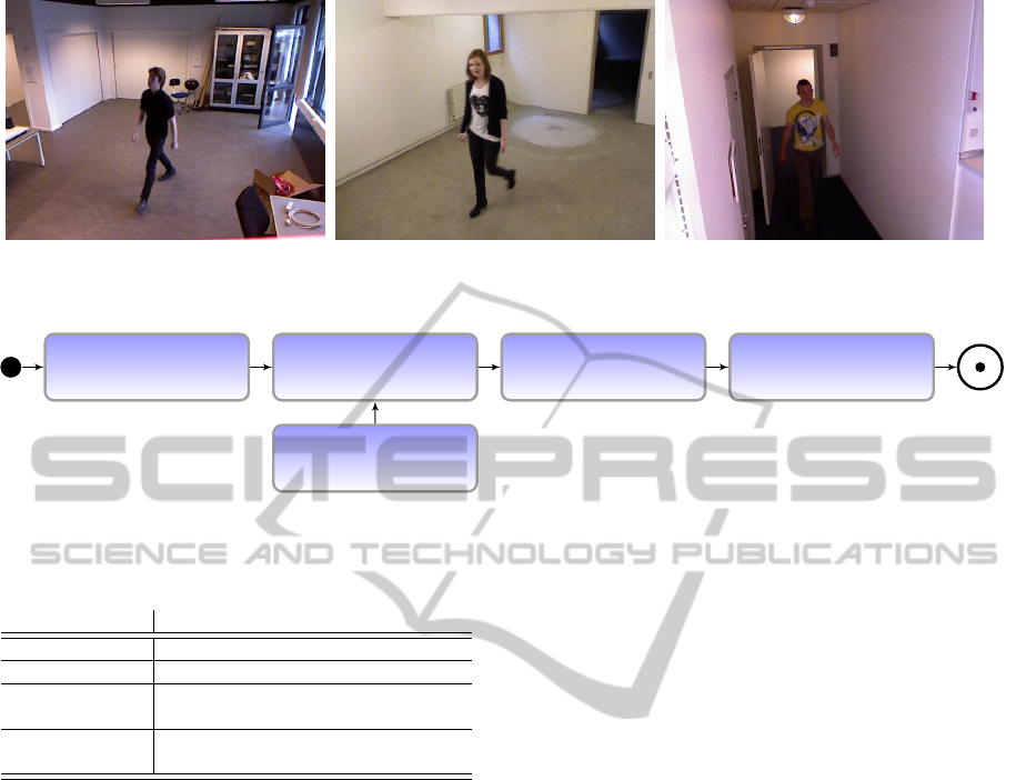
(a) (b) (c)
Figure 1: Example images from our own (a) Novi, (b) Basement, and (c) Hallway sequences.
Detection
Segmentation
Ground plane
estimation
Generate model
Re-identification
Figure 2: Illustration of the flow through the system.
Table 1: Statistics on the three data sequences used in this
work.
Novi Basement Hallway
Number of persons 22 35 10
Number of frames 7800 7231 4492
Contains image se-
quences
Yes Yes Yes
Available modalit-
ies
RGB, depth RGB, depth,
thermal
RGB, depth,
thermal
3 ALGORITHM OVERVIEW
This paper describes a full re-identification system
which takes a raw RGB-D feed as input and outputs
whether or not a passing person has been seen before,
and if so, what the previous ID was. This is different
from many other re-identification papers which most
often describe a core algorithm without much focus
on all the other system parts that must be in place to
have an actual working system. The process requires
several steps: Persons must be detected and segmen-
ted, they must be modeled, and finally re-identified.
On top of the re-identification process comes the pro-
cess of keeping tabs on the person database. A flow-
chart is shown in fig. 2.
3.1 Detection and Segmentation
The detection is done with a standard HOG-detector
as first proposed by Dalal and Triggs (Dalal and
Triggs, 2005). The detector is trained on the INRIA
Person Dataset introduced by the same paper. The
detector runs on the RGB images and returns person
bounding boxes.
The detected persons need to be segmented in fur-
ther detail. The bounding box is not sufficient, since
we do not want to capture features from the back-
ground. Segmentation is achieved with a flood fill in
the depth image. Persons not crawling on the floor
are conveniently separated from the background in the
depth modality, so a flood fill to similar pixels starting
at the points
X =
2/5 1/4
2/5 1/3
2/5 2/5
1/2 1/4
1/2 1/3
1/2 2/5
3/5 1/4
3/5 1/3
3/5 2/5
b
w
0
0 b
h
+
b
x
b
y
.
.
.
.
.
.
b
x
b
y
9x2
(1)
where X is a 9x2 matrix containing the x and y co-
ordinates of the flood fill points, b is the bounding
box with subscript x, y, w, and h meaning top-left
x-coordinate, top-left y-coordinate, width, and height
respectively. The flood fill is performed at multiple
positions to ensure that we have a stable object in the
depth modality. A person is classified as stable if at
least j depth points converge, i.e. the flood fill of these
points fill out the same volume. For this implementa-
tion, j = 4.
VISAPP2015-InternationalConferenceonComputerVisionTheoryandApplications
246
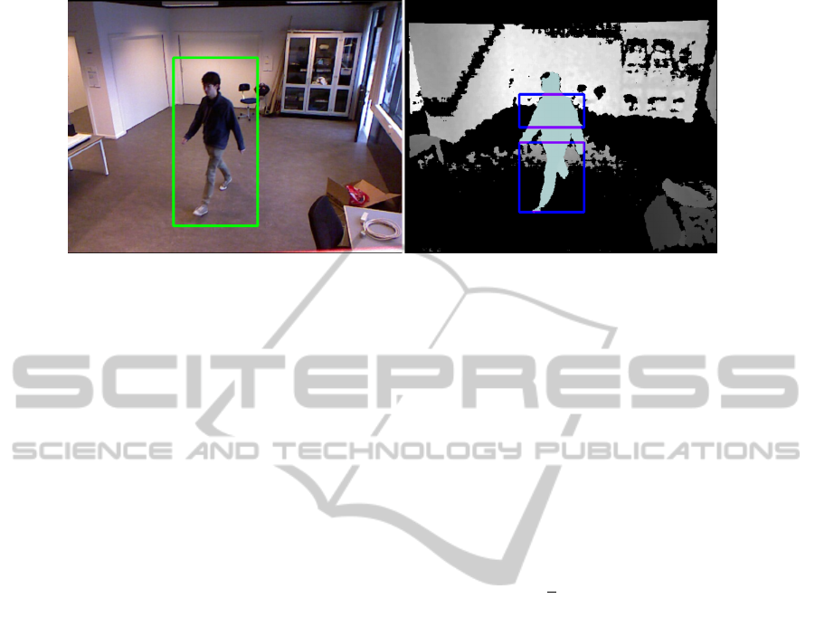
Figure 3: The left image illustrates a detection. On the right, the person has been segmented in the depth image, and the blue
boxes illustrates the boxes which are used as basis for the color histograms.
3.1.1 Ground Plane Estimation
One problem with the flood fill is that at the feet of
the subject, the fill is likely to spill onto the floor. To
counter this, ground plane pixels on the depth image
are removed. When the system is started initially, a
ground plane is defined in the depth image. This is
done by marking a number of points on the ground
and performing a least squares solution of the bivari-
ate polynomial:
z
poly
= a
00
+a
01
x +a
02
x
2
+a
10
y+a
20
y
2
+a
11
xy (2)
Although the floor is planar, the measurements of the
floor from the Kinect depth sensor are representing
the plane as a hyperbolic plane, thus stating the need
for a bivariate polynomial. When the coefficients are
determined, any pixel in the depth image close to the
ground plane is colored black. Those pixels are the
ones fulfilling the inequality in equation (3), where
p is the pixel in question and t
depth
defines the dis-
tance from the theoretical ground plane that is still
considered part of that plane.
|z
poly
− p
z
| < t
depth
(3)
3.2 Person Model
One of the objectives of this paper is to compare two
types of multi-shot person models. They are both
based on the two-part color histogram used in (Mø-
gelmose et al., 2013b): After a person is segmented, a
color histogram is computed for the upper part of the
body and the lower part of the body (as illustrated by
the blue boxes in fig. 3). Each color channel is di-
vided into 20 bins, the individual channel histograms
are concatenated, and finally the two part histograms
are concatenated for a feature vector of 20 ·3 ·2 = 120
dimensions in the case of a 3 channel color space. In
addition to the two modeling paradigms, 3 different
color spaces were tested: RGB, HSV, and XYZ. For
HSV and XYZ the luminance channels were removed
to enhance lighting invariance, so in those cases the
final histogram would be 80-dimensional and contain
just the HS- and XZ-channels, respectively.
Two multi-shot schemes have been tested:
1) Mean histogram of all frames in a pass.
2) All frame-histograms saved individually.
In 1) the mean histogram is computed when a pass
is over. Each bin is simply averaged:
m
i
=
1
n
n
∑
j=0
h
i, j
for 0 ≤ i < k (4)
where m is the mean histogram, n is the number of
frames in the pass, k is the number of bins in the his-
tograms and h
i, j
is the value of bin i in histogram j.
In 2) no averaging takes place. Instead a pass is
modeled after each histogram in it. See the follow-
ing section on how each model is matched against the
person database.
Both of the color-based models are augmented
with a measure of the person’s height. We use normal-
ized height-to-border. This is the distance in pixels
from the top of the person in the image, to the bottom
of the frame, normalized by the depth of the observa-
tion. This reduces noise, as only one of the bounds
of the height is now determined from the noisy depth
sensor. It also allows for clipping.
In fig. 4 height-to-border versus depth is plotted.
Because the surface and field-of-view is the same for
all who pass by the camera, the only change that will
happen to the curve for people of different heights is
a shift in its y-axis intercept. Instead of approximat-
ing the full curve, we go for the less computationally
heavy option of modelling each pass with the mean
of the depth-normalized height-to-border, designated
γ, for all instances in the pass:
ComparisonofMulti-shotModelsforShort-termRe-identificationofPeopleusingRGB-DSensors
247

Figure 4: Curves depicting height-to-border versus distance
for all tracks in a sequence. The curves are colored in pairs,
such that two tracks of the same color are two passes by
the same person. It can be seen that most lines are close
to their partner of the same color, showing that the height
measurement is stable across passes.
γ =
1
n
n
∑
i=0
g
i
· d
i
(5)
where g
i
is the height-to-border for observation i in
the pass, and d
i
is the distance to the person in that
observation. While the person is not completely flat,
for the purpose of this normalization, we use the depth
of the seed point described in equation 1.
3.3 Re-identification
A pruning stage based on the height measurement is
used before the re-identification. The height of the
probe is compared to the gallery by means of the ab-
solute difference in their heights. If the mean normal-
ized height-to-border is more than t
h
away from a can-
didate, the candidate is not considered a match for this
subject. t
h
is found from analyzing training data be-
fore running the system. The threshold t
h
is set to the
mean of the height difference between wrong matches
in the training set.
When re-identifying, the model of the current pass
is compared to those of the persons in the database,
which is initially empty, but will be built as time pro-
gresses. Both the mean histogram and the histogram
series model use the Bhattachariyya distance (Bradski
and Kaehler, 2008):
d(H
1
,H
2
) =
s
1 −
∑
I
p
H
1
(I)H
2
(I)
p
∑
I
H
1
(I) ·
∑
I
H
2
(I)
(6)
where d(H
1
,H
2
) is the distance between the histo-
grams H
1
and H
2
, and H(I) is the value of bin I in
the histogram H. The result is a number between 0
and 1, where 0 is a perfect match.
With mean histograms, where only two histo-
grams - probe and gallery - are involved, the distance
itself is used, and the subject is either re-identified,
ignored, or added to the database. With histogram
series, the model comprise a series of histograms. In
this case, each histogram in the probe model is com-
pared to each histogram in the database. The probe
then casts a vote for the ID of the gallery-model which
contains the histogram it is closest to, if that is within
a separately trained ignore threshold. The gallery-
model with the most votes is selected as the best can-
didate, provided is has the majority (more than 50%)
of the possible votes.
3.4 Mean Histogram
The re-identification process is overned by two
thresholds:
t
n
: New threshold: Subjects with d(H
1
,H
2
) > t
n
are added as new persons
(7)
t
i
: Ignore threshold: Subjects with d(H
1
,H
2
) <= t
i
are re-identified
(8)
This implicates that subjects with t
i
< d(H
1
,H
2
) <=
t
n
are ignored, because they are too similar to other
subjects, without being similar enough to trust the
identification.
The thresholds are learned beforehand by ob-
serving a training set. The distances between all mean
histograms in the training set are computed and stored
in the set D and divided into two sets D
c
and D
w
where D
c
contains distances between different obser-
vations of the same person and D
w
contains distances
between histograms of different persons:
D
c
= {D|id(H
1
) = id(H
2
) in d(H
1
,H
2
)} (9)
D
w
= {D|id(H
1
) 6= id(H
2
) in d(H
1
,H
2
)} (10)
where id(•) is the person id connected with a his-
togram. The thresholds are then computed as:
t
n
= D
w
− 2 · σ(D
w
) (11)
t
i
= D
c
+ σ(D
c
) (12)
where • denotes mean and σ(•) denotes standard
deviation.
3.5 Histogram Series
The re-identification for the histogram series model
uses many of the same principles of the mean histo-
gram model, but is adapted to use many more his-
tograms for each subject to encompass variations in
VISAPP2015-InternationalConferenceonComputerVisionTheoryandApplications
248

lighting and pose. A histogram is computed for each
frame in the pass of a subject and they are then com-
pared to all histograms already in the database. When
the shortest distance d
s
to any gallery-histogram is
less than t
i
, the associated person id, p
s
receives a
vote. Thus, each subject histogram contributes with
up to 1 vote, for a theoretical total of len(H) votes:
the number of histograms in the current pass. If there
are no histograms in the pass, the subject is ignored. If
any person in the gallery has received more than half
the theoretical maximum, the subject is re-identified
as him. If no gallery person satisfies this requirement,
the subject is added as a new person.
It is worth noting that this method has no explicit
option of ignoring the subject in case it is uncertain,
other than in the case where no histograms exist.
4 EVALUATION
6 permutations of the system have been tested on 3
different sequences (see section 2.1). The 2 differ-
ent multi-shot models have both been tested in 3 dif-
ferent color spaces: RGB, HSV, and XYZ.HSV and
XYZ have been tested since they both model color
closer to how the human eye sees it, and more spe-
cifically because they allow for exclusion of the lu-
minance so that differing lighting conditions should
affect performance less. That means that for the fol-
lowing tests all three RGB channels were used, in the
HSV case only HS were used, and with XYZ only XZ
were used.
The performance of the system varies with the or-
der the persons are passing by the camera. If a person
that is very hard to re-identify passes by the camera
in the first two passes without any other entries in
the database, odds are that he will be correctly re-
identified. However, if a similar person enters the
database before the second pass of person 1, they
might be confused with each other and thus lower
the performance. To even out this effect, all res-
ults presented below are averages of 100 runs where
the subjects enters the system in random order. That
should sufficiently even out any “lucky” or “unlucky”
orderings and provide accurate results. For each run,
all thresholds have been trained on a random subset of
20% of the sequence, which is then excluded from the
rest of the run. The effect of the training set selection
should also average out.
The re-identification performance can be charac-
terized with 5 parameters:
1. Correct new
2. Wrong new
3. Correct ID
4. Wrong ID
5. Ignored
The first two describes how well the system dis-
tinguishes between known persons and new persons.
Ideally, there should be no wrong new, as they are per-
sons that are already in the database and should have
been re-identified. Correct ID and wrong ID com-
prises the subjects that are neither ignored, correct
new, nor wrong new, but are re-identified. Finally, ig-
nored are the ones that are not handled because they
are neither close enough to an existing person to be
re-identified, nor different enough from the existing
persons to be added to the database.
The results of the tests can be seen in table 3.
Sequence length and detection performance varies
greatly between sequences, as seen in table 2. Note
that the Hallway sequence contains many shorter
tracks, meaning that generalization, as well as the be-
nefit from the multi-shot approach, declines heavily.
Generally, the mean histogram and histogram
series approaches perform equally when looking at
the percentage rates of the identification. The differ-
ences between the two approaches are most profound
in the Basement and Novi sequences. The histogram
series approach contains no ignore category which
leads to a higher number of wrong new identifications
than compared with the mean histograms. However,
the method returns a significantly lower number of
wrong identifications in both sequences. It is seen
from the standard deviation of that the mean histo-
gram exhibits a more stable performance than the his-
togram series on correct identifications whereas the
opposite seems to be the case for wrong identifica-
tions. The number of wrong identifications is low
across the board, so the weak spots are the wrong
new- and ignored-counts which are rather high. Most
new passes are correctly classified as such, at around
29-32 of 35 in the basement sequence, 8/10 and 21/22
in the Hallway and Novi sequences respectively.
The benefit of the ignore-functionality in the mean
histogram model is illustrated in fig. 5. Blue columns
are a histogram of distances between mean histo-
grams of the same person, while red columns are
a histogram of distances between different persons.
The overlap between these shows that is it not pos-
sible to achieve perfect classification with a 1d de-
cision boundary in this case. To counter this, an ig-
nore zone is introduced - the space between the green
and the yellow line, the thresholds, which can to some
extent mitigate the effects of this overlap. In real-
ity, when training on a subset of the data, the ignore
zones are generally wider than in this example. It is
possible that a classification in a higher dimensional
ComparisonofMulti-shotModelsforShort-termRe-identificationofPeopleusingRGB-DSensors
249

Table 2: Statistics on the amount of observations of captured persons for each sequence. The numbers are based on the amount
of times a single person was detected and modeled in a single pass.
Basement seq. Hallway seq. Novi seq.
Mean observation length: 25.5 10.3 40.7
Median observation length: 24 11.5 41
Minimum observation length: 4 2 5
Maximum observation length: 38 25 57
Table 3: Re-identification performance of the 6 system configurations on 3 different sequences. All numbers are averaged
over 100 runs with random enrollment order. The standard deviation of the results are shown in parenthesis.
Basement sequence
Correct new Wrong new Correct ID Wrong ID Ignored % correct % wrong
RGB
Mean histogram 29.31 (2.92) 4.53 (7.10) 11.76 (5.34) 1.22 (2.50) 8.18 (6.82) 90.62 % 9.38 %
Histogram series 32.61 (1.44) 8.64 (7.37) 13.00 (7.07) 0.74 (2.14) 0.00 (0.00) 94.60 % 5.40 %
HS
Mean histogram 28.75 (3.23) 3.20 (7.36) 12.57 (5.81) 1.18 (2.83) 9.30 (6.78) 91.43 % 8.57 %
Histogram series 32.71 (1.37) 8.13 (7.77) 13.49 (7.51) 0.67 (2.27) 0.00 (0.00) 95.24 % 4.76 %
XY
Mean histogram 29.02 (3.26) 4.72 (7.12) 11.24 (5.15) 1.68 (3.01) 8.34 (7.35) 86.97 % 13.03 %
Histogram series 32.54 (1.45) 8.88 (7.34) 12.59 (6.87) 0.98 (2.33) 0.00 (0.00) 92.78 % 7.22 %
Hallway sequence
Correct new Wrong new Correct ID Wrong ID Ignored % correct % wrong
RGB
Mean histogram 8.36 (1.00) 4.07 (2.34) 1.15 (1.37) 0.61 (1.01) 0.81 (1.62) 65.34 % 34.66 %
Histogram series 8.59 (0.77) 4.45 (2.10) 1.30 (1.57) 0.66 (1.18) 0.00 (0.00) 66.33 % 33.67 %
HS
Mean histogram 8.15 (1.17) 3.95 (2.41) 1.34 (1.61) 0.39 (0.78) 1.17 (2.13) 77.46 % 22.54 %
Histogram series 8.61 (0.62) 4.44 (2.14) 1.44 (1.72) 0.51 (0.76) 0.00 (0.00) 73.85 % 26.15 %
XY
Mean histogram 8.37 (0.96) 4.11 (2.29) 1.15 (1.37) 0.63 (1.10) 0.74 (1.58) 64.61 % 35.39 %
Histogram series 8.57 (0.71) 4.33 (2.14) 1.37 (1.58) 0.73 (1.22) 0.00 (0.00) 65.24 % 34.76 %
Novi sequence
Correct new Wrong new Correct ID Wrong ID Ignored % correct % wrong
RGB
Mean histogram 21.15 (1.40) 3.79 (2.98) 9.68 (2.73) 0.25 (1.31) 1.13 (1.89) 97.48 % 2.52 %
Histogram series 21.51 (0.70) 9.12 (4.21) 5.31 (4.24) 0.06 (0.42) 0.00 (0.00) 98.88 % 1.12 %
HS
Mean histogram 20.64 (1.86) 2.42 (2.13) 10.52 (2.38) 0.44 (1.45) 1.98 (3.21) 95.99 % 4.01 %
Histogram series 21.48 (0.77) 9.18 (4.53) 5.23 (4.59) 0.11 (0.91) 0.00 (0.00) 97.94 % 2.06 %
XY
Mean histogram 21.14 (1.17) 4.89 (3.48) 8.83 (3.10) 0.34 (1.26) 0.80 (1.74) 96.29 % 3.71 %
Histogram series 21.46 (0.87) 10.12 (3.91) 4.31 (3.93) 0.11 (0.91) 0.00 (0.00) 97.51 % 2.49 %
Table 4: Comparison of re-identification performance with and without the height-based candidate pruning step.
Without height With height Difference
% correct % wrong % correct % wrong % correct % wrong
Basement
Mean histogram 82.17 % 17.83 % 90.67 % 9.33 % 8.50 % -8.50 %
Histogram series 87.28 % 12.72 % 94.21 % 5.79 % 6.93 % -6.93 %
Hallway
Mean histogram 64.64 % 35.36 % 69.14 % 30.86 % 4.50 % -4.50 %
Histogram series 67.34 % 32.66 % 68.47 % 31.53 % 1.10 % -1.10 %
Novi
Mean histogram 92.03 % 7.97 % 96.59 % 3.41 % 4.56 % -4.56 %
Histogram series 96.50 % 3.51 % 98.11 % 1.89 % 1.61 % -1.61 %
Average 81,66 % 18,34 % 86,20 % 13,80 % 4,53 % -4.53 %
space would work better and allow discarding the ig-
nore zone.
Table 4 shows how the height-based pruning step
improves the re-id rates across all methods. By dis-
carding obviously wrong candidates based on height,
the correct re-id rate goes up by 4.53 percentage
points on average.
We have been unable to compare our results to the
work of others, as they do not present full-flow sys-
tems, but rely on tightly pre-cropped images of per-
sons. Furthermore, our system needs depth images as
well as RGB, so no existing dataset has been com-
patible. We also do not present CMC-curves as that
ranking system works poorly for on-the-fly enroll-
ment systems, where, in many cases, there are simply
not enough entries in the database to do a proper rank-
ing.
We can, however, compare some of our results to
VISAPP2015-InternationalConferenceonComputerVisionTheoryandApplications
250

Figure 5: Distribution of distances between histograms in
the full basement sequence. There is a clear overlap of dis-
tances between histograms from the same person and his-
tograms from different persons. When using a distance
threshold to classify, this will result in wrong identifica-
tions. The ignore-threshold allows to remove the distances
that are the most affected by this overlap.
the work previously presented in (Møgelmose et al.,
2013b). Not all stats are directly comparable, but the
correct and wrong ID rates are. In that work, they are
68% and 0%, with an ignore rate of 24%. The system
presented here has a much higher correct ID rate, but
at the cost of a somewhat higher wrong ID rate.
5 CONCLUSION
This work presented a re-identification system using
RGB-D data and compared several model and color
space configurations. It introduces 3 new, different re-
identification sequences for testing, and goes through
all stages from candidate detection to identification.
Furthermore, it investigates how to handle online en-
rollment of subjects, a subject few previous works
have touched. Future work includes more sophistic-
ated multi-shot models, and enhancing the system to
cope with multiple, co-occluding subjects in crowded
environments.
REFERENCES
Bak, S., Charpiat, G., Corvée, E., Brémond, F., and Thon-
nat, M. (2012). Learning to Match Appearances by
Correlations in a Covariance Metric Space. In ECCV
(3), volume 7574 of LNCS, pages 806–820. Springer.
Barbosa, I. B., Cristani, M., Bue, A. D., Bazzani, L., and
Murino, V. (2012). Re-identification with RGB-D
Sensors. In ECCV Workshops (1), volume 7583 of
LNCS, pages 433–442. Springer.
Bradski, G. and Kaehler, A. (2008). Learning OpenCV,
chapter 7, pages 201–202. O’Reilly.
Dalal, N. and Triggs, B. (2005). Histograms of Oriented
Gradients for Human Detection. In CVPR.
Demirkus, M., Garg, K., and Guler, S. (2010). Automated
person categorization for video surveillance using soft
biometrics. pages 76670P–76670P–12.
Doretto, G., Sebastian, T., Tu, P. H., and Rittscher, J. (2011).
Appearance-based person reidentification in camera
networks: problem overview and current approaches.
J. Ambient Intelligence and Humanized Computing,
2(2):127–151.
Jüngling, K. and Arens, M. (2010). Local Feature Based
Person Reidentification in Infrared Image Sequences.
In AVSS, pages 448–455. IEEE Computer Society.
Møgelmose, A., Clapés, A., Bahnsen, C., Moeslund, T. B.,
and Escalera, S. (2013a). Tri-modal Person Re-
identification with RGB, Depth and Thermal Features.
In 9th IEEE Workshop on Perception Beyond the Vis-
ible Spectrum. IEEE.
Møgelmose, A., Moeslund, T. B., and Nasrollahi, K.
(2013b). Multimodal Person Re-Identification using
RGB-D Sensors and a Transient Identification Data-
base. In International Workshop on Biometrics and
Forensics.
Velardo, C. and Dugelay, J. (2012). Improving Identifica-
tion by Pruning: A Case Study on Face Recognition
and Body Soft Biometric. In WIAMIS, pages 1–4.
IEEE.
Zhao, R., Ouyang, W., and Wang, X. (2013). Unsuper-
vised Salience Learning for Person Re-identification.
CVPR.
Zheng, W., Gong, S., and Xiang, T. (2011). Person re-
identification by probabilistic relative distance com-
parison. In CVPR, pages 649–656. IEEE.
ComparisonofMulti-shotModelsforShort-termRe-identificationofPeopleusingRGB-DSensors
251
