
Models for Multimodal Freight Transportation Integrating
Consolidation and Transportation Phases
Leonardo Malta
1
, Nicolas Jozefowiez
1
and Fr
´
ederic Semet
2
1
LAAS-CNRS, Toulouse, France
2
Ecole Centrale de Lille, Lille, France
Keywords:
Intermodal Transportation, Freight Consolidation, Mixed-Integer Programming.
Abstract:
It is important for economic development and international trade the ability to move freight in a cost-efficient,
safe and quick fashion. The paper will discuss the door-to-door freight transportation problem in its two
phases: consolidation phase and transportation between the platforms. In a general way, the problem is de-
scribed as a set of orders that have a release and delivery date and must be consolidated and routed from
a source to a destination point. Two models are proposed, both integrating several aspects of the problem
such as long-haul transportation, freight consolidation, freight storage and intermodal transportation. The first
is a time-space based model and the second an implicit time representation model. Models are formulated
as integer programming problems and some results of small practical instances are shown along with some
considerations.
1 INTRODUCTION
Intermodal transportation can be loosely defined as
the movement of goods from a source to a destination
using a transportation network composed of several
modes (rail, truck, road and so on). Seeking to reduce
operations costs, meet customer requirements for im-
proved service and the increasing volume of freight
itself, the industry has to consolidate their freight in a
network of hubs and terminals with regular services.
This consolidation is made in a standardized way to
decrease the complexity and improve the efficiency
of these operations.
Several papers have been devoted to the subject
in the past few years. The chapters dedicated to in-
termodal transportation (Crainic and Kim, 2007) and
maritime transportation (Christiansen et al., 2007) are
reviews on the subject covering the literature up to
2005. Another review can be found in (SteadieSeifi
et al., 2014) focusing recent works on the subject.
These reviews present papers covering strategic, tacti-
cal and operational aspects of the problem. This work
relates more closely with the ones focused on the tac-
tical planning aspect of the problem. At this level
the goal is to optimize the use of a given infrastruc-
ture by choosing services and modes and allocating
their capacities to orders. For a tactical level stand-
point review, we refer to (Wieberneit, 2007). Even
at this level several approaches can be taken, focus-
ing on different elements. For instance, (Anghinolfi
et al., 2011) proposes a path-based approach that also
consider the allocation of containers to trains wagon
and (Shintani et al., 2007) integrates empty container
repositioning.
The closest related papers to our work are (Ayar
and Yaman, 2011; Bauer et al., 2010). On (Ayar
and Yaman, 2011), the goal is to reduce contain-
ers transportation and storage cost using a combina-
tion of trucks and maritime transportation. They also
consider fixed scheduled vehicles and capacity con-
straints. On (Bauer et al., 2010) a time-space model
is proposed to design a network with the goal of min-
imizing greenhouse gas emissions. Although, the fo-
cus is more on a strategic rather than tactical level, a
similar time-space model is used on our work.
Most of the work on intermodal transportation
deals with the movement of already consolidated con-
tainers. In this paper, we focus on the integration of
the consolidation and transportation phase. In other
words, the problem faced combines two main deci-
sion: the first one is to assign orders to containers, the
second one is the transportation of containers them-
selves. An important aspect to notice in our problem
is the fixed schedule of vehicles. In other words, all
the routes and departure/arrival dates are known a pri-
ori.
338
Malta L., Jozefowiez N. and Semet F..
Models for Multimodal Freight Transportation Integrating Consolidation and Transportation Phases.
DOI: 10.5220/0005210803380345
In Proceedings of the International Conference on Operations Research and Enterprise Systems (ICORES-2015), pages 338-345
ISBN: 978-989-758-075-8
Copyright
c
2015 SCITEPRESS (Science and Technology Publications, Lda.)
This paper is organized as follows. The Section 2
gives a general description of the problem. Section 3
presents two integer programming models proposed
for the problem. Section 4 shows tests results com-
paring both models. Section 5 gives the conclusion
and our perspectives for the future of the work.
2 PROBLEM DESCRIPTION
We are given a set of transportation requests (orders),
which should be picked up from their origins at given
release time and should be delivered to their destina-
tions no later than their due dates. These orders are
taken to a consolidation terminal at their origin to be
grouped (or assigned into containers). A container is
closed and ready for transportation only after the re-
lease date of every order assigned to it. It is important
to note that containers in this case are just logical enti-
ties with the purpose of grouping orders. They them-
selves do not have the traditional source/destination
pair or a release and delivery dates.
Once the consolidation takes place, containers are
ready to be transported to its destination consolidation
terminal. The transportation happens using scheduled
services (vehicles) of a given mode (rail, ships, etc).
Each service has a time-window when it is possible to
load containers to it. That way, for a container to use a
service, it must be closed and ready for transportation
at the location as the load time-window takes place. It
is possible to transfer containers between different ve-
hicles/modes during the transportation. Furthermore,
it is possible to transport a container directly from
source to destination using on demand trucks (direct
transportation). Finally, there is a limit on the num-
ber of containers transported by each vehicle (trans-
portation capacity), the number of containers stored
at a given location (storage capacity) and a limit on
how many orders can be assigned to a same container
(container capacity). Each container operation (trans-
port, storage and vehicle transfer) has a cost associ-
ated with it and the goal is to minimize the overall
cost for the transportation of every order to its desti-
nation.
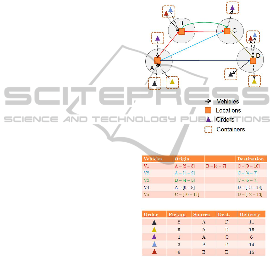
A small example is shown in Figure 1. In this ex-
ample, there are three location A, B, C and D con-
nected by five vehicles. Vehicles schedules can be
view on the top table in Figure 2. On the bottom ta-
ble five orders, represented by colored triangles, are
presented with their source, destination, pickup and
delivery dates. The dashed boxes are used to repre-
sent the grouping/assignment of orders to containers
prior to their transportation. In this example, we can
notice that even when orders have the same source
and destination, they sometimes cannot be assigned
to the same container due to their release and dead-
line dates. That is the case of orders represented by
the yellow and black triangles in the example.
Figure 1: Small example representation.
Figure 2: Small example data.
3 MODELING THE PROBLEM
This study proposes an integrated approach by de-
signing two 0-1 integer programming models to find a
solution to our problem. The first model uses a time-
space network which is a intuitive and easy way to
represent the problem. The second model makes use
of the fact that vehicles schedules are known before-
hand and represent the time horizon implicitly.
ModelsforMultimodalFreightTransportationIntegratingConsolidationandTransportationPhases
339
3.1 Time-space Model
The time-space network representation divides the en-
tire time horizon considered into a set T of time pe-
riods t
1
, . . . ,t
max
of equal length. This is a straightfor-
ward and traditional way to represent connection be-
tween vehicles and storage operations. The notation
used by this model are the following:
Locations and Time
Two nodes are defined for each location at every time
period: storage and consolidation nodes. Consoli-
dation nodes are used to represent the consolidation
phase of the problem.
• N - set of locations in the network.
• Q
n
- storage capacity of a location n ∈ N .
• σ
n
- storage terminal for a location n ∈ N .
• γ
n
- consolidation terminal for a location n ∈ N .
• T - set of time periods comprising the time hori-
zon considered.
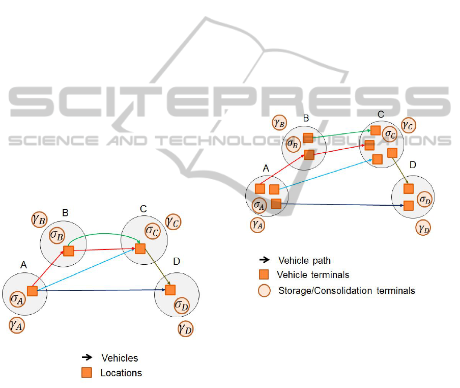
In Figure 3 we illustrate the addition of consoli-
dation and storage terminals for each location used in
the small example presented in Figure 1.
Figure 3: Addition of consolidation and storage terminals
Vehicles
Each vehicle is represented by a different graph. Each
node on its graph represent a terminal for that specific
vehicle and corresponds, but is not equal, to a location
in the network. The arcs of the graph represent the
vehicle path. We also assume that a vehicle departs
from (or arrives to) a terminal exactly after (or before)
the load/unload time interval.
• V - set of vehicles connecting network locations.
• G
v
= (N
v
, A
v
) - graph representing the vehicle v ∈
V .
• Each i ∈ N
v
- a terminal for that specific vehicle v
at a location in N .
• η
i
∈ N - location of terminal i
• ν
i
∈ V - vehicle to which terminal i belongs.
• ϒ
i
v
⊂ T - load/unload time interval at terminal i ∈
N
v
.
• (i, j) ∈ A
v
- path segment of a vehicle.
• A
T
= ∪
v∈V
A
v
- all transportation arcs.
In Figure 4 we illustrate each vehicle terminal rep-
resented by a separated orange box. The arrows in the
Figure, representing vehicle paths, connect only ter-
minals belonging to a single vehicle.
Figure 4: Separate graph for each vehicle.
Storage and Vehicle Transfer
Storage and transfer operations can take place at each
location. To represent this, we divide all vehicle ter-
minals in two sets, one for terminals where a vehicle
departs from a location and a load operation can take
place and other for terminals where a vehicle arrives
to a location and a unload operation can happen. Note
that a terminal can be part of both sets in case of a in-
termediate stop in the vehicle path.
• N
+
= {i|(i, j) ∈ A
v
, v ∈ V } - set of departure ter-
minals.
• N
−
= {i|( j, i) ∈ A
v
, v ∈ V } - set of arrival termi-
nals.
• N
S
= {σ
n
|n ∈ N } - set of all storage terminals.
ICORES2015-InternationalConferenceonOperationsResearchandEnterpriseSystems
340
• N
C
= {γ
n
|n ∈ N } - set of all consolidation termi-
nals.
To define arcs representing vehicle transfer opera-
tions, we must notice that this operation can happen
only from an arrival terminal to a departure one (of
different vehicles), provided that the load/unload in-
terval of both terminals coincide. Storage arcs are de-
fined in three different types. First, the unloading of
a container from a arrival terminal to a storage termi-
nal. Second, the loading of a container from a storage
terminal to a departure terminal. And finally, from
a storage terminal to the same storage terminal (con-
tainer stays stored).
• A
M
= {(i, j)|i ∈ N
−
, j ∈ N
+
, η
i
= η
j
, ν
i
6= ν
j
} -
vehicle transfer arcs.
• A
S
in
= {(i, σ
n
)|i ∈ N
+
, η
i
= n} - unloading arcs.
• A
S
out
= {(σ
n
, i)|i ∈ N
−
, η
i
= n} - loading arcs.
• A
S
stored
= {(σ
n
, σ
n
)} - storage arcs.
• A
S
= A
S
in
∪ A
S
out
∪ A
S
stored
- all storage arcs.
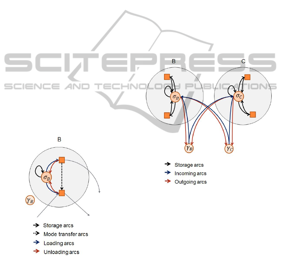
To illustrate these definitions, we can zoom in a
location from the example in Figure 1. Figure 5 show
the unloading arcs A
S
in
(red arrows), unloading arcs
A
S
in
(blue arrows), storage arcs A
S
stored
(black arrows)
and vehicle transfer arcs (dashed arrows) for location
B.
Figure 5: Arcs representing storage and vehicle transfers
operations for location B.
Direct Transportation
To represent direct transportation of containers we de-
fine a set of arcs from a consolidation terminal to each
storage terminal (incoming arcs) and the other way
around (outgoing arcs). In other words, these arcs rep-
resent that a container is closed (at the consolidation
terminal) and is ready for transportation at its source
storage terminal or at a storage terminal in another lo-
cation (using on demand trucks). Similarly, arcs form
a storage terminal to a consolidation terminal repre-
sent that a container arrives at its destination.
• I = {(γ
n
, σ
m
)|n, m ∈ N }
• O = {(σ
n
, γ
m
)|n, m ∈ N }
Figure 6 illustrates this in the example of Figure
1. We show only two of the locations (B and C) of the
example to simplify the illustration. The incoming
arcs are represented by blue arrows, going from each
consolidation terminal to each storage terminal. Out-
going arcs are represented by red arrows and connect
each storage terminal to each consolidation terminal.
Figure 6: Incoming and outgoing operations for locations B
and C.
Time Periods
Finally, we add time dimension to our definitions. For
each time period t ∈ T , we define G
t
= (N
t
, A
t
) as a
graph representing the network at period t, where:
• N
t
= N
+
t
∪ N
−
t
∪ N
S
t
, ∀t ∈ T - set of all nodes at
period t.
• A
T
t
= {(i, j, t)|(i, j) ∈ A
v
, v ∈ V, δ
i j
= t} - set of
arcs representing all transportation that happens
at period t.
• A
S
in
t
= {(i, j,t)|(i, t) ∈ N
S
t
, ( j,t) ∈ N
+
t
, η
i
= η
j
} -
unloading arcs at period t.
• A
S
out
t
= {(i, j,t)|(i, t) ∈ N
−
t
, ( j,t) ∈ N
S
t
, η
i
= η
j
} -
loading arcs at period t.
ModelsforMultimodalFreightTransportationIntegratingConsolidationandTransportationPhases
341

• A
S
stored
t
= {(i, j,t)|(i, t) ∈ N
S
t
, ( j,t + 1) ∈
N
S
t+1
, η
i
= η
j
} - storing arcs at period t.
• A
S
t
= A
S
in
t
∪ A
S
out
t
∪ A
S
stored
t
- all storage arcs.
• A
M
t
= {(i, j, t)|i ∈ N
−
t
, j ∈ N
+
t
, η
i
= η
j
, ν
i
6= ν
j
,t ∈
ϒ
i
v
∩ ϒ
j
v
}, set of mode transfer terminals at period
t.
• A
t
= A
T
t
∪ A
S
t
∪ A
M
t
- mode transfers arcs at period
t.
• I∗ = {(γ
n
, σ
m
,t)|n, m ∈ N ,t ∈ T } - set of all in-
coming arcs.
• O∗ = {(σ
n
, γ
m
,t)|n, m ∈ N ,t ∈ T } - set of all out-
going arcs.
The complete time-space network is, then, the union
of each period graph G = (N, A), where:
• N = ∪
t∈T
(N
+
t
∪ N
−
t
∪ N
S
t
∪ N
C
t
)
• A = ∪
t∈T
A
t
∪ I ∗ ∪O∗
Finally, each arc in the graph has the following pa-
rameters:
• c
i j
- cost of a transport, storage or transfer opera-
tion between terminal i and j.
• Q
i j
- operation capacity (in numbers of contain-
ers).
• ∆
i j
- time taken to perform operation.
Orders and Containers
Moreover, we define the set of orders and the set of
containers. In this model, we do not manage empty
containers movement. We assume there is a container
available to each order (both sets have the same size).
• L - the set of orders
• K - set of containers.
• s
l
, d
l
∈ N - the source and destination location of
the order.
• φ
l
, ω
l
∈ T - the pickup and delivery date.
• w
l
- the weight of the order.
• Q
k
the capacity of a container k.
Model
We can now describe the entire model:
Minimize:
∑
a
t
i j
∈A
∑
k∈K
c
i j
x
t
i jk
(1)
Subject to:
∑
k∈K
y
lk
= 1 ∀l ∈ L (2)
∑
l∈L
w
l
y
lk
≤ Q
k
∀k ∈ K (3)
∑
a
t
ii
∈A
S
∑
k∈K
x
t
iik
≤ Q
n
∀t ∈ T , n ∈ N , i = σ
n
(4)
∑
k∈K
x
t
i jk
≤ Q
i j
∀a
t
i j
∈ A\A
S
(5)
∑
φ
l
≤t≤ω
l
a
t
i j
∈I
x
t
i jk
≥ y
lk
∀l ∈ L, ∀k ∈ K, i = γ
s
l
(6)
∑
φ
l
≤t≤ω
l
a
t
i j
∈O
x
t
i jk
≥ y
lk
∀l ∈ L, ∀k ∈ K, j = γ
d
l
(7)
∑
a
t−∆
i j
ji
∈A
∑
k∈K
x
t
jik
−
∑
a
t
i j
∈A
∑
k∈K
x
t
i jk
= 0 ∀i ∈ N\N
C
(8)
∑
a
t
i j
∈I
x
t
i jk
≤ 1 ∀k ∈ K (9)
∑
a
t
i j
∈O
x
t
i jk
≤ 1 ∀k ∈ K (10)
y
lk
∈ {0, 1}, ∀l ∈ L, ∀k ∈ K (11)
x
t
i jp
∈ {0, 1} ∀a
t
i j
∈ A (12)
The variables y
lk
are assignment variables to indicate
if order l is assigned to container k and x
t
i jk
are trans-
portation variables to indicate if container k travels
through an arc at period t. The objective function 1 is
the operation cost minimization.
Constraint 2 ensures every order is assigned to a
container. Next constraints concern with capacity of
elements. Constraint 3 ensures the number of orders
assigned to a container respects its capacity. Con-
straint 4 ensures the number of containers traveling
through all storage arcs A
S
at a given location is be-
low its storage capacity. And constraint 5 are capacity
on transportation or transfers operations.
Constraint 6 ensures the departure of a con-
tainer from the consolidation terminal of its as-
signed orders and also ensures time restrictions
(pickup/delivery date). Constraint 7 is analogous to
6 for the arrival of containers. Constraints 8 and 9 en-
sures containers enter and exit the network only once.
3.2 Implicit Time Representation
As we can expect, the main drawback of a time-space
representation is how it scales with the size of the time
horizon. The model grows very fast the more periods
it considers. Nonetheless, since the schedule infor-
mation for all vehicles are known a priori, the repre-
sentation of time can be made implicitly avoiding a
ICORES2015-InternationalConferenceonOperationsResearchandEnterpriseSystems
342
complete discretization of it. To achieve this, most of
changes on the previous model are very straightfor-
ward but a more careful effort during the definition
of the graph representing the transportation network
(specially, the mode transfer arcs) is required. Instead
of defining a set of transportation variables for each
time period, we define variables to indicate if a con-
tainer is transported between locations using a given
vehicle.
Location storage capacity representation cannot
be made without some bigger changes, though. The
reason for this is that we no longer define a single
variable to indicate if a container is stored at a spe-
cific period as in the time-space model. Then, we
have to find a way to discretize time so that at any
given period storage capacity is ensured. However, as
it is known the arrival and departure date for each ve-
hicle, it is also possible to know how long a container
must be stored if transported by a given vehicle. We
consider that a container can be stored either if it has
just been closed (and waits for transportation) or if is
is being transferred from a vehicle to another.
The events that can potentially change the the
number of containers stored at a location are the ar-
rival or departure of vehicles. So we can divide time
based on these events and define sets Λ of arcs rep-
resenting vehicle transfers occurring between them.
Thus, these sets contain arcs that simultaneously re-
quire storage resources. The idea is represented in
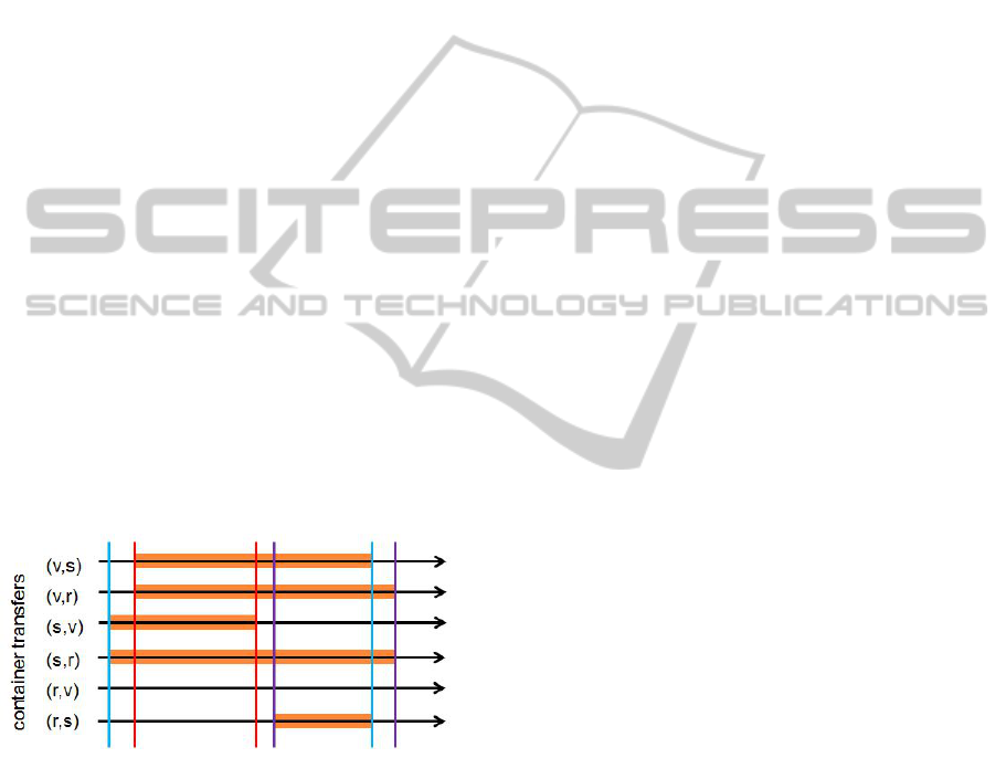
Figure 7.
Figure 7: Example of storage time for vehicle transfers.
The timeline represent the possible container transfers
at a hypothetical location n. The colored lines repre-
sent the arrival and departure date for three vehicles
(red: vehicle v, blue: vehicle s and purple: vehicle r).
The orange box represents the storage time required
to transfer a container. The first line, for instance, il-
lustrates a container storage time for a transfer from
vehicle v to vehicle s. The first red line represents the
arrival of vehicle v and the second blue line the depar-
ture of vehicle s.
To define the set of transfers that requires simul-
taneously storage resources we observe the timeline
and take the first vehicle arrival event (e
1
). Next, we
take the first vehicle departure event (d
1
) that occurs
after e
1
. Every arc that requires storage (orange box)
between e
1
and d
1
is added to a new set Λ
1
n
for the
location n. We repeat the process by taking the next
arrival event and the departure event after it until no
more events lasts.
Let
¯
Λ
n
= {Λ
1
n
, Λ
2
n
, . . . , Λ
i
n
} be the set of all sets de-
fined for a location n. The pseudo-algorithm to iden-
tify these sets can be described the following way:
1. Let e
v
, be the arrival date of a vehicle v at location
n. Let d
v
, be the departure date of a vehicle v at
location n
2. Let
¯
Λ
n
=
/
0.
3. Let t
a
= t
d
= 0, let i = 1.
4. If there is a vehicle arrival t
d
< e
v
, then t
a
= e
v
else end the algorithm.
5. If there is a vehicle departure t
a
< d
v
, then t
d
= d
v
else end the algorithm.
6. Let Λ
i
n
be the set of all transfers the requires stor-
age resources between periods t
a
and t
d
7.
¯
Λ
n
=
¯
Λ
n
∪ Λ
i
n
, i = i + 1
8. Go to step 4.
On the example of Figure 3 the first arrival event
is from vehicle s (e
1
) and the first departure event
after it is from vehicle v (d
1
). All transfers that
happen between these events are added to set Λ
1
n
=
{(v, s), (v, r), (s, v)(s, r)}. The first arrival event af-
ter d
1
is from vehicle r (e
2
) and first departure
event after it is from vehicle s (d
2
). This results
in Λ
2
n
= {(v, s), (v, r), (s, r)(r, s)}. So the algorithm
yields
¯
Λ
n
= {Λ
1
n
, Λ
2
n
} for location n.
The storage constraint can be defined as:
∑
a
t
i j
∈Λ
i
n
∑
k∈K
x
i jk
≤ Q
n
n ∈ N , ∀Λ
i
n
∈
¯
Λ
n
This constraints ensures that the number of containers
stored simultaneously (represented by the sets con-
tained in
¯
ϒ
n
) does not violate location storage capac-
ity. The complete model is described below:
Minimize:
∑
a
i j
∈A
∑
k∈K
c
i j
x
i jk
(13)
∑
k∈K
y
lk
= 1 ∀l ∈ L (14)
∑
l∈L
w
l
y
lk
≤ Q
k
∀k ∈ K (15)
∑
a
i j
∈ϒ
i
n
∑
k∈K
x
i jk
≤ Q
n
n ∈ N , ∀Λ
i
n
∈
¯
Λ
n
(16)
ModelsforMultimodalFreightTransportationIntegratingConsolidationandTransportationPhases
343
∑
k∈K
x
i jk
≤ Q
i j
∀a
i j
∈ A\A
S
(17)
∑
a
i j
∈I
x
i jk
≥ y
lk
∀l ∈ L, ∀k ∈ K, i = σ
s
l
(18)
∑
a
i j
∈O
x
i jk
≥ y
lk
∀l ∈ L, ∀k ∈ K, i = σ
d
l
(19)
∑
a
ji
∈A
∑
k∈K
x
jik
−
∑
a
i j
∈A
∑
k∈K
x
i jk
= 0 ∀i ∈ N\N
C
(20)
∑
a
i j
∈I
x
i jk
≤ 1 ∀k ∈ K (21)
∑
a
i j
∈O
x
i jk
≤ 1 ∀k ∈ K (22)
y
lk
∈ {0, 1}, ∀l ∈ L, ∀k ∈ K (23)
x
i jp
∈ {0, 1} ∀a
i j
∈ A (24)
Variables and constraints remain similar to the
ones on the previous model, without the time dimen-
sion. The variables y
lk
are assignment variables to in-
dicate if order l is assigned to container k and x
i jk
are
transportation variables to indicate if container k trav-
els through an arc. The objective function 13 remains
the operation cost minimization.
Constraint 14 ensures every order is assigned to a
container. Next constraints concern with capacity of
elements. Constraint 15 ensures the number of orders
assigned to a container respects its capacity. Con-
straint 16 ensures the number of containers traveling
through all storage arcs A
S
at a given location is below
its storage capacity. And constraint 17 are capacity on
transportation or transfers operations.
Constraint 18 ensures the departure of a con-
tainer from the consolidation terminal of its as-
signed orders and also ensures time restrictions
(pickup/delivery date). Constraint 19 is analogous to
18 for the arrival of containers. Constraints 20 and
21 ensures containers enter and exit the network only
once.
4 RESULTS
Two sample transportation networks were designed.
One consisting of 6 locations, 20 vehicles serving
them and a time horizon of 25 time periods. The
second, consisting of 4 locations, 12 vehicles and a
time horizon of 40 time periods. Random generated
instances were also created with 10, 12 and 15 or-
ders. Tests were made on a Intel Core i5-3570 3.4
GHz and 4Gb of RAM. The solver used was ILO
CPLEX v12.4. Table 1 shows the results obtained
for the time taken to find a solution and model size
in terms of number of variable and constraints for the
time-space model (TSM) and the implicit time rep-
resentation model (ITRM). The percentage values in
the solution time column represent the size of the opti-
mality gap when stopping the solver after 20 minutes
of running time.
Table 1: Results for randomly created instances and 6 loca-
tions.
TSM ITRM
time(s) var const time(s) var const
10 orders
test1 20.98 7739 49774 2.64 1210 10870
test2 9%* 7853 50364 14.4 1230 12280
test3 911.08 6965 46754 6.65 1110 11700
test4 3.51 7439 48414 98.39 1230 11470
test5 45.47 7082 46724 5.5 1230 11410
12 orders
test6 11%* 9638 60936 35.64 1613 14136
test7 18%* 9722 60996 124.74 1674 15084
test8 32%* 9650 60960 51.09 1691 14880
test9 11.19 9734 60948 212.1 1736 14916
test10 59.97 9710 60948 5.41 1751 15684
15 orders
test11 82.58%* 12302 76209 69.09 2338 19395
test12 43.21%* 12332 76299 32.25 2355 20325
test13 65.34%* 12392 76239 1276.19 2477 19545
test14 44.54%* 12392 76224 5%* 2429 19680
test15 8.24%* 12482 76224 3%* 2567 20580
Table 2: Results for randomly created instances and 4 loca-
tions.
TSM ITRM
time(s) var const time(s) var const
10 orders
test1 5%* 8677 51560 0.3 620 3150
test2 55.4 8288 50430 0.7 640 3260
test3 48.3 8249 50340 0.5 620 2870
test4 3 8341 50630 0.4 620 3000
test5 112.6 8084 49130 0.2 630 3120
12 orders
test6 11.5%* 10628 62100 0.2 836 4284
test7 26.3 10580 62112 0.2 860 4080
test8 41.87%* 10508 62112 0.2 848 3540
test9 5 10592 62100 2.1 836 3636
test10 39 10532 62100 0.3 848 4008
15 orders
test11 42.6%* 13574 77670 4.2 1112 5190
test12 61.4%* 13634 77685 0.4 1142 5310
test13 30.0%* 13529 77730 1 1142 4560
test14 11.6 13634 77670 0.8 1112 4815
test15 56.2%* 13454 77670 14.5 1142 5055
Few points can be noticed. First, the addition of very
few orders to the problem greatly increases model size
and time taken to find a solution. On the network hav-
ing 6 locations, for most instances having more than
15 orders, both models could not finish calculations
due to memory restrictions. Second, implicit time
representation indeed reduces number of constraints
and variables significantly, proportionally to the num-
ber of periods considered. Most of the time this re-
duction leads to a shorter solution time, but that is not
always the case. This can be seen in results of tests 4
and 9. Third, there is a great variation of the solution
time for instances of the same size. And an interest-
ICORES2015-InternationalConferenceonOperationsResearchandEnterpriseSystems
344

ing point for research is to explore how the structure
of an instance can influence solution time. Finally, the
integration of consolidation and transportation phases
make freight transportation problem a lot harder. For
comparison, if we pre-assign order to containers (by
fixing variables) and thus not considering the consol-
idation phase, both models can find solution for in-
stances with 100 order in a few seconds.
5 CONCLUSION
Freight transportation is an important and complex
domain to be studied. In this paper we have presented
the initial study on the integration of consolidation
and transportation phase. We have proposed two 0-
1 integer programming models for the problem. The
first model is a time-space model whereas the sec-
ond represent time implicitly. The discretization of
time used by the time-space model allows to easily
add more features to the problem (pre-consolidation
storage cost, multi-drop capabilities, etc) whereas the
second model has the advantage of being capable to
consider a longer time horizon. The initial results ob-
tained from both approaches shows that the integra-
tion of phases makes freight transportation problem
harder.
Several research points can be explored from this
initial work. The large size of the problem suggests
the use of decomposition methods, such as column
generation. Moreover, the result suggests that the in-
stance structure can have a great influence on solu-
tion times and a formal description of this relation
is needed. Finally, since transportation industry may
have different concerns besides economical costs (en-
vironmental, QoS, etc), it is desirable to include mul-
tiple objectives to the model.
REFERENCES
Anghinolfi, D., Paolucci, M., Sacone, S., and Siri, S.
(2011). Freight transportation in railway networks
with automated terminals: A mathematical model and
MIP heuristic approaches. European Journal of Op-
erational Research, 214(3):588–594.
Ayar, B. and Yaman, H. (2011). An intermodal mul-
ticommodity routing problem with scheduled ser-
vices. Computational Optimization and Applications,
53(1):131–153.
Bauer, J., Bektas, T., and Crainic, T. G. (2010). Minimiz-
ing greenhouse gas emissions in intermodal freight
transport: an application to rail service design. JORS,
61(3):530–542.
Christiansen, M., Fagerholt, K., Nygreen, B., and Ronen, D.
(2007). Handbooks in Operations Research and Man-
agement Science, volume Volume 14, chapter Chapter
4 Maritime Transportation, pages 189–284. Elsevier.
Crainic, T. G. and Kim, K. H. (2007). Handbooks in Op-
erations Research and Management Science, volume
Volume 14, chapter Chapter 8 Intermodal Transporta-
tion, pages 467–537. Elsevier.
Shintani, K., Imai, A., Nishimura, E., and Papadimitriou, S.
(2007). The container shipping network design prob-
lem with empty container repositioning. Transporta-
tion Research Part E: Logistics and Transportation
Review, 43(1):39–59.
SteadieSeifi, M., Dellaert, N., Nuijten, W., Van Woensel, T.,
and Raoufi, R. (2014). Multimodal freight transporta-
tion planning: A literature review. European Journal
of Operational Research, 233(1):1–15.
Wieberneit, N. (2007). Service network design for freight
transportation: a review. OR Spectrum, 30(1):77–112.
ModelsforMultimodalFreightTransportationIntegratingConsolidationandTransportationPhases
345
