
Improvement of Recovering Shape from Endoscope Images Using RBF
Neural Network
Yuji Iwahori
1
, Seiya Tsuda
1
, Robert J. Woodham
2
, M. K. Bhuyan
3
and Kunio Kasugai
4
1
Dept. of Computer Science, Chubu University, Kasugai 487-8501, Japan
2
Dept. of Computer Science, University of British Columbia, Vancouver V6T 1Z4, Canada
3
Dept. of Electronics and Electrical Engineering, Indian Institute of Technology Guwahati, Guwahati 781039, India
4
Dept. of Gastroenterology, Aichi Medical University, Nagakute 480-1195, Japan
Keywords:
Endoscope Image, VBW Model, RBF-NN, Shape Modification, Reflection Factor.
Abstract:
The VBW (Vogel-Breuß-Weickert) model is proposed as a method to recover 3-D shape under point light
source illumination and perspective projection. However, the VBW model recovers relative, not absolute,
shape. Here, shape modification is introduced to recover the exact shape. Modification is applied to the output
of the VBW model. First, a local brightest point is used to estimate the reflectance parameter from two images
obtained with movement of the endoscope camera in depth. After the reflectance parameter is estimated, a
sphere image is generated and used for Radial Basis Function Neural Network (RBF-NN) learning. The NN
implements the shape modification. NN input is the gradient parameters produced by the VBW model for
the generated sphere. NN output is the true gradient parameters for the true values of the generated sphere.
Depth can then be recovered using the modified gradient parameters. Performance of the proposed approach
is confirmed via computer simulation and real experiment.
1 INTRODUCTION
Endoscopy allows medical practitioners to observe
the interior of hollow organs and other body cavi-
ties in a minimally invasive way. Sometimes, diag-
nosis requires assessment of the 3-D shape of the ob-
served tissue. For example, the pathologicalcondition
of a polyp often is related to its geometrical shape.
Medicine is an important area of application of com-
puter vision technology. Specialized endoscopes with
a laser light beam head (Nakatani et al., 2007) or with
two cameras mounted in the head (Mourgues et al.,
2001) have been developed. Many approaches are
based on stereo vision (Thormaehlen et al., 2001).
However, the size of the endoscope becomes large
and this imposes a burden on the patient. Here, we
consider a general purpose endoscope, of the sort still
most widely used in medical practice.
Shape recovery from endoscope images is consid-
ered. Shape from shading (SFS) (Horn, 1975) and
Fast Marching Method (FMM) (Sethian, 1996) based
SFS approach (Kimmel and Sethian, 2001) are pro-
posed. These approaches assume orthographic pro-
jection. An extension of FMM to perspective projec-
tion is proposed in (Yuen et al., 2007). Further ex-
tension of FMM to both point light source illumina-
tion and perspective projection is proposed in (Iwa-
hori et al., 2010). Recent extensions include gener-
ating a Lambertian image from the original multiple
color images (Ding et al., 2010), (Neog et al., 2011).
Application of FMM includes solution (Iwahori et al.,
2014) under oblique illumination using neural net-
work learning (Ding et al., 2009). Most of the pre-
vious approaches treat the reflectance parameter as a
known constant. The problem is that it is impossible
to estimate the reflectance parameter from only one
image. Further, it is also difficult to apply point light
source based photometric stereo (Iwahori et al., 1990)
in the context of endoscopy.
Iwahori et al. (Iwahori et al., 1997) developed Ra-
dial Basis Function Neural Network (RBF-NN) pho-
tometric stereo, exploiting the fact that an RBF-NN
is a powerful technique for multi-dimensional non-
parametric functional approximation.
Recently, the Vogel-Breuß-Weickert (VBW)
model (Vogel et al., 2007), based on solving the
Hamilton-Jacobi equation, has been proposed to re-
cover shape from an image taken under the conditions
of point light source illumination and perspective
62
Iwahori Y., Tsuda S., Woodham R., Bhuyan M. and Kasugai K..
Improvement of Recovering Shape from Endoscope Images Using RBF Neural Network.
DOI: 10.5220/0005206800620070
In Proceedings of the International Conference on Pattern Recognition Applications and Methods (ICPRAM-2015), pages 62-70
ISBN: 978-989-758-077-2
Copyright
c
2015 SCITEPRESS (Science and Technology Publications, Lda.)

projecction. However, the result recovered by the
VBW model is relative. VBW gives smaller values
for surface gradient and height distribution compared
to the true values. That is, it is not possible to apply
the VBW model directly to obtain exact shape and
size.
This paper proposes a new approach to improve
the accuracy of polyp shape determination as absolute
size. The proposed approach estimates the reflectance
parameter from two images with small camera move-
ment in the depth direction. A Lambertian sphere
model is synthesized using the estimated reflectance
parameter. The VBW model is applied to the synthe-
sized sphere and shape then is recovered. An RBF-
NN is used to improve the accuracy of the recovered
shape, where the input to the NN is the surface gradi-
ent parameters obtained with the VBW model and the
output is the corresponding, corrected true values.
The proposed approach is evaluated via computer
simulation and real experiments and it is confirmed
that the obtained shape is improved.
2 VBW MODEL
The VBW model (Vogel et al., 2007) is proposed as a
method to calculate depth (distance from the viewer)
under point light source illumination and perspective
projection. The method solves the Hamilton-Jacobi
equations (Benton, 1977) associated with the models
of Faugeras and Prados (Prados and Faugeras, 2004)
(Prados and Faugeras, 2003). Lambertian reflectance
is assumed.
The following processing is applied to each point
of the image. First, the initial value for the depth
Z
default
is given using Eq.(1) as in (Prados and
Faugeras, 2005).
Z
default
= −0.5log(I f
2
) (1)
where I represents the normalized image intensity and
f is the focal length of the lens.
Next, the combination of gradient parameters
which gives the minimum gradient is selected from
the difference of depths for neighboring points. The
depth, Z, is calculated from Eq.(2) and the process
is repeated until the Z values converge. Here, (x, y)
are the image coordinates, ∆t is the change in time,
(m, n) is the minimum gradient for (x, y) directions,
and Q =
f
√
x
2
+y
2
+ f
2
is the coefficient of the perspec-
tive projection.
Z(x, y) = Z(x, y) + ∆t exp(−2Z(x, y))
−∆t
I f
2
Q
√
f
2
(m(x)
2
+n(y)
2
)+(xm(x)+yn(y))
2
+Q
2
(2)
Here, it is noted that the shape obtained with the
VBW model is given in a relative scale, not an abso-
lute one. The obtained result gives smaller values for
surface gradients than the actual gradient values.
3 PROPOSED APPROACH
3.1 Estimating Reflectance Parameter
When uniform Lambertian reflectance and point light
source are assumed, image intensity depends on the
dot product of surface normal vector and the light
source direction vector subject to the inverse square
law for illuminance.
Measured intensity at each surface point is deter-
mined by Eq.(3).
E = C
(s·n)
r
2
(3)
where E is image intensity, s is a unit vector towards
the point light source, n is a unit surface normal vec-
tor, and r is the distance between the light source and
surface point.
The proposed approach estimates the value of the
reflectance parameter, C, using two images acquired
with a small camera movement in the depth direc-
tion. It is assumed that C is constant for all points
on the Lambertian surface. Regarding geometry, it is
assumed that both the point light source and the op-
tical center of lens are co-located at the origin of the
(X, Y, Z) world coordinate system. Perspective pro-
jection is assumed.
The actual endoscope image has the color textures
and specular reflectance. Using the approach pro-
posed by (Shimasaki et al., 2013) the original input
endoscope image is converted into one that satisfies
the assumptions of a uniform Lambertian gray scale
image.
The procedure to estimate C is as follows.
Step 1. If the value of C is given, depth Z is uniquely
calculated and determined at the point with the lo-
cal maximum intensity (Tatematsu et al., 2013).
At this point, the surface normal vector and the
light source direction vector are aligned and pro-
duce the local maximum intensity for that value
of C.
Step 2. For camera movement, ∆Z, in the Z direction,
two images are used and the difference in Z, Z
dif f
,
at the local maximum intensity points in each im-
age is calculated. Here the camera movement, ∆Z,
is assumed to be known.
ImprovementofRecoveringShapefromEndoscopeImagesUsingRBFNeuralNetwork
63
Step 3. Let f(C) be the error between ∆Z and Z
dif f
.
f(C) represents an objective function to be min-
imized to estimate the correct value of C. That
is, the value of C is the one that minimizes f (C)
given in Eq.(4).
f(C) = (∆Z −Z
dif f
(x, y))
2
(4)
3.2 NN Learning for Modification of
Surface Gradient
The size and shape recovered by the VBW model are
relative. VBW gives smaller values for surface gra-
dient and depth compared to the true values. Here,
modification of surface gradient and improvement of
the recovered shape are considered. First, the sur-
face gradient at each point is modified by a neural
network. Then the depth is modified using the esti-
mated reflectance parameter,C, and the modified sur-
face gradient, (p, q) = (
∂Z
∂X
,
∂Z
∂Y
). A Radial Basis Func-
tion Neural Network (RBF-NN) (Ding et al., 2009) is
used to learn the modification of the surface gradient
obtained by the VBW model.
Using the estimated C, a sphere image is synthe-
sized with uniform Lambertian reflectance.
The VBW model is applied to this synthesized
sphere. Surface gradients, (p, q), are obtained using
forward difference of the Z values obtained from the
VBW model.
The estimated gradients, (p, q), and the corre-
sponding true gradients for the synthesized sphere,
(p, q), are given respectively as input vectors and out-
put vectors to the RBF-NN. NN learning is applied.
After NN learning, the RBF-NN can be used to
modify the recovered shape for other images.
Two endoscope images, (a) and (b), and the im-
ages assuming Lambertian reflectance, (c) and (d),
generated using (Shimasaki et al., 2013), are shown
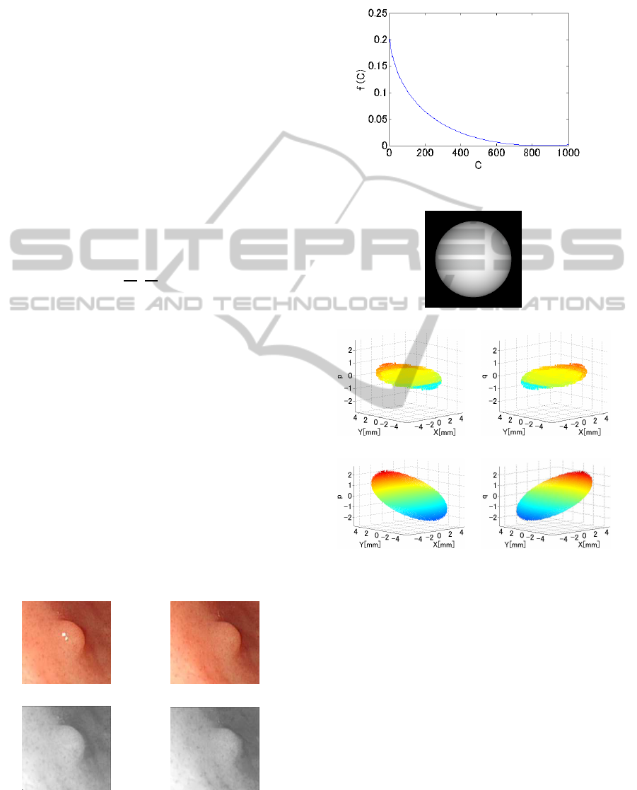
(a) Orginal1 (b) Orginal2
(c) Lambert1 (d) Lambert2
Figure 1: Endoscope Image and Lambertian Image.
in Fig.1.
An example of the objective function, f(C), is
shown in Fig.2.
Figure 2: Objective Function f(C).
(a) Sphere
(b) p by VBW (c) q by VBW
(d) True p (e) True q
Figure 3: Synthesized Sphere for NN Learning.
The synthesized sphere image used in NN learn-
ing is shown in Fig.3(a). Surface gradients obtained
by the VBW model are shown in Fig.3(b)(c) and the
correspondingtrue gradients for this sphere are shown
in Fig.3(d)(e). Points are sampled from the sphere as
input for NN learning, except for points with large
values of (p, q). The procedure for NN learning is
shown in Fig.4.
3.3 NN Generalization and
Modification of Z
The trained RBF-NN allows generalization to other
test objects. Modification of estimated gradients,
ICPRAM2015-InternationalConferenceonPatternRecognitionApplicationsandMethods
64
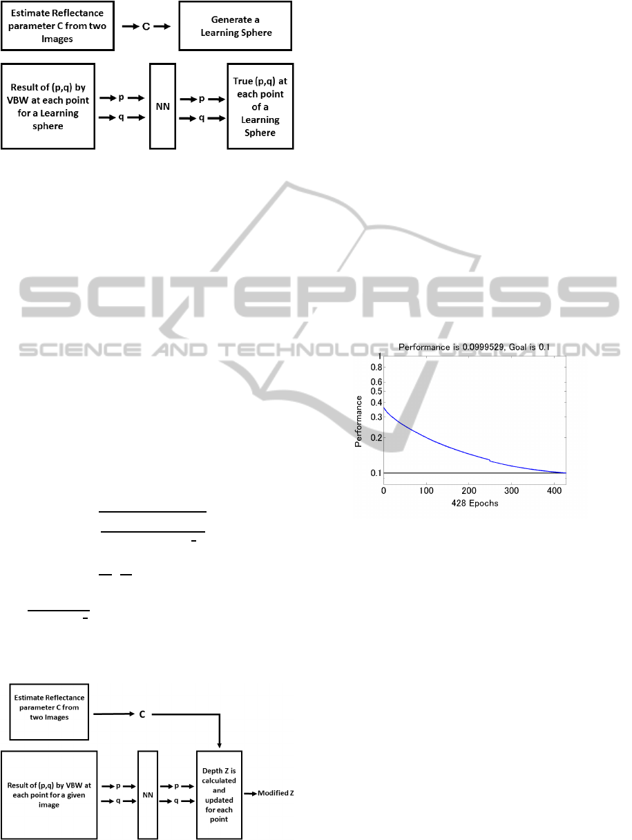
Figure 4: Learning Flow.
(p, q), is applied to the test object and its depth, Z, is
calculated and updated using the modified gradients,
(p, q).
In the case of endoscope images, preprocessing is
used to remove specularities and to generate a uni-
form Lambertian image based on (Shimasaki et al.,
2013).
Next, the VBW model is applied to the this Lam-
bertian image and the gradients, (p, q), are estimated
from the obtained Z distribution.
The estimated gradients, (p, q), are input to the
NN and modified estimates of (p, q) are obtained as
output from the NN.
Recall that the reflectance parameter, C, is esti-
mated from f(C), based on two images obtained by
small movement of endoscope in the Z direction.
The depth, Z, is calculated and updated by Eq.(5)
using the modified gradients, (p, q), and the estimated
C, where Eq.(5) also is the original equation devel-
oped in (Iwahori et al., 2010).
Z =
s
CV(−px−qy+ f)
E(p
2
+ q
2
+ 1)
1
2
(5)
Again, (p, q) = (
∂Z
∂X
,
∂Z
∂Y
), E represents image inten-
sity, f represents the focal length of the lens and
V =
f
2
(x
2
+y
2
+ f
2
)
3
2
.
A flow diagram of the processing described above
is shown in Fig.5.
Figure 5: Flow of NN Generalization.
4 EXPERIMENTAL RESULTS
4.1 NN Learning
A sphere was synthesized with radius 5mm and with
center located at (0, 0, 15). The focal length of the
lens was 10mm. The image size was 9mm×9mm
with pixel size 256×256 pixels.
The VBW model was used to recover the shape of
this sphere. The resulting gradient estimates, (p, q),
are shown in Fig.3(b) and (c), respectively.
These estimated gradients, (p, q), are used as NN
input and the corresponding true gradients, (p, q),
output from the NN, are shown in Fig.3(d) and (e).
Learning was done under the conditions: error goal
1.0e-1, spread constant of the radial basis function
0.00001, and maximum number of learning epochs
500. Learning was complete by about 400 epochs
with stable status.
The results of learning is shown in Fig.6.
Figure 6: Learning Result.
The reflectance parameter, C, was estimated as
854 from f (C). The difference in depth, Z, was 0.5
[mm] for the known camera movement.
As shown in Fig.6, NN learning was complete at
428 epochs. The square error goal reached the spec-
ified value. Processing time for NN learning was
around 30 seconds.
A sphere has a variety of surface gradients and it
is used for the NN learning. After a sphere is used for
NN learning, not only a sphere object but also other
object with another shape including convex or con-
cave surfaces is also available in the generalization
process. This is because surface gradient for each
point is modified by NN and this modification does
not depend on the shape of target object.
4.2 Computer Simulation
Computer simulation was performed for a second pair
of synthesized images to confirm the performance of
ImprovementofRecoveringShapefromEndoscopeImagesUsingRBFNeuralNetwork
65
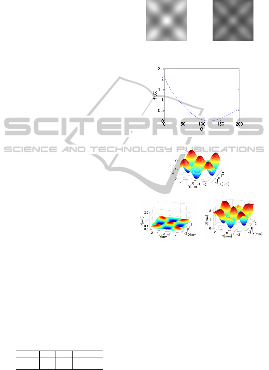
NN generalization. Synthesized cosine curved sur-
faces were used, one with center located at coordi-
nates (0, 0, 12) and the other with center at (0, 0, 15).
Common to both, the reflectance parameter,C, is 120,
the focal length, f, is 10mm and the waveform cycle
is 4mm and the ± amplitude is 1mm. Image size is
5mm×5mm and pixel size is 256×256 pixels.
The synthesized image whose center is located at
(0, 0, 12) is shown in Fig.7(a) and the one with center
located at (0, 0, 15) is shown in Fig.7(b).
The reflectance parameter, C, was estimated ac-
cording to the proposed method. Using the learned
NN, the gradients, (p, q), obtained from the VBW
model were input and generalized. The gradients,
(p, q), were modified and the depths, Z, were updated
using Eq.(5).
The graph of the objective function, f(C), is
shown in Fig.8 and the true depth is shown in Fig.9(a).
The estimated C was 119 (compared to the true value
of 120). The estimagtd Z
dif f
was 2.9953 (compared
to the true value of 3).
The result recovered by VBW for Fig.7(a) is
shown in Fig.9(b). The modified values of depth, us-
ing the NN and Eq.(5), are shown in Fig.9(c).
Table.1 gives the mean errors in surface gradient
and depth estimation. The percentages given in the
Z column represent the error relative to the amplitude
of maximum−minimum depth (=4mm) of the cosine
synthesized function. In Table 1, the original VBW
results have a mean error of around 3.8 degrees for the
surface gradient while the proposed approach reduced
the mean error to about 0.1 degree. Depth estimation
also improved to a mean error of 8.3% from 43.1%.
NN generalization improved estimation of shape for
an object with different size and shape. It took 9 sec-
onds to recover the shape while it took 61 seconds for
NN learning with 428 learning epochs, that is, it took
70 seconds in total.
Computer simulation was performed for a sec-
ond pair of synthesized images to confirm the per-
formance of NN generalization. Synthesized cosine
curved surfaces were used, one with center located at
coordinates (0, 0, 12) and the other with center at (0,
0, 15). Common to both, the reflectance parameter,C,
is 120, the focal length, f, is 10mm and the waveform
cycle is 4mm and the ± amplitude is 1mm.
Another experiment was performed under the fol-
lowing assumptions. The reflectance factor,C, is 590,
Table 1: Mean Error.
p q Z[mm]
VBW 23.04 23.04 0.86 (43.1%)
Proposed 0.32 0.32 0.25 ( 8.3%)
(a) Center:(0,0,12) (b) Center:(0,0,15)
Figure 7: Cosine Model.
Figure 8: Objective Function f(C).
(a) True Z
(b) Z by VBW (c) Modified Z
Figure 9: Results.
the focal length, f, is 10mm and the object is a sphere
with radius 5mm. The centers for two positions of the
sphere were set at (0, 0,15) and (0, 0, 17) respectively,
as shown in Fig.10. The image size was 9mm× 9mm
with pixel size 360×360 pixels. Here, 4% Gaus-
sian noise (mean 0, variance 0.02, standard deviation
0.14142) is added to each of the two input images.
The graph of the objective function, f(C), is shown in
Fig.11 and the true depth is shown in Fig.12(a). The
result recovered by VBW is shown in Fig.12(b). The
improved result is shown in Fig.12(c). The mean er-
rors in surface gradient and depth are shown in Table
2. Evaluations for 6% (mean 0, variance 0.03, stan-
dard deviation 0.17320) and 10% (mean 0, variance
0.03, standard deviation 0.17320) Gaussian noise in-
cluded in Table 3, as well.
ICPRAM2015-InternationalConferenceonPatternRecognitionApplicationsandMethods
66
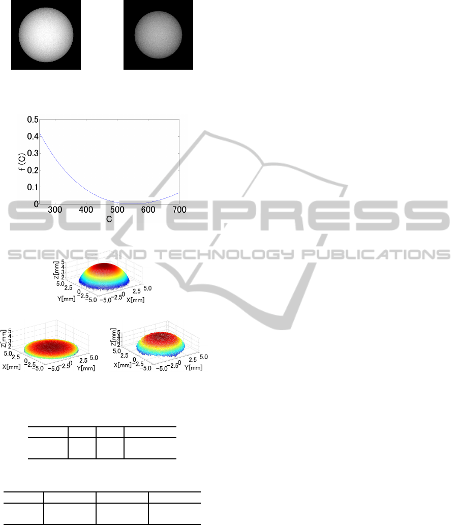
(a) Center:(0,0,15) (b) Center:(0,0,17)
Figure 10: Sphere Images with Gaussian Noise.
Figure 11: Objective Function f (C).
(a) True Z
(b) Z by VBW (c) Modified Z
Figure 12: Results.
Table 2: Mean Error.
p q Z[mm]
VBW 17.04 17.45 3.36 (67.2%)
Proposed
0.45 0.45 0.36 ( 7.2%)
Table 3: Mean Error of Z for Different Gaussian Noise.
4% 6% 10%
VBW 3.36 (67.2%) 3.25 (65.1%) 2.82 (56.6%)
Proposed
0.36 ( 7.2%) 0.36 ( 7.2%) 0.36 ( 7.3%)
Learning epochs for Gaussian noise 4%, 6% and
10% were 212, 212 and 210. Processing time was
around 40 seconds for every case of different Gaus-
sian noises.
The reflectance parameter, C, estimated from
Fig.11, was 591. Improvement in the estimated re-
sults is shown in Fig.12(a)(b)(c) and Table 2.
In all three cases, Gaussian noise of 4%, 6% and
10%, the proposed approach reduced the mean er-
ror in Z significantly compared to the original VBW
model.
This suggests generalization using the RBF-NN is
robust to noise and is applicable to real imaging sit-
uations, including endoscopy. Result of VBW model
gives less errors with noises butthis is based on the re-
sult that the recovered shape is relative scale and sen-
sitive to the original intensity of each point according
to Gaussian noise, while the proposed approach gives
much better shape with the absolute size. Although
the error increases a little bit according to Gaussian
noise, the approach is still robust and stable result is
obtained.
4.3 Real Image Experiments
Two endoscope images obtained with camera move-
ment in the Z direction are used in the experiments.
The reflectance parameter,C, was estimated and a
RBF-NN was learned using a sphere synthesized with
the estimated C. VBW was applied to one of the im-
ages which was first converted to a uniform Lamber-
tian image.
Surface gradients, (p, q), were modified with the
NN then depth, Z, was calculated and updated at each
image point. The focal length, f=10mm, the image
size 5mm×5mm, and camera movement, ∆Z=3mm,
were assigned to the same known values as those in
the computer simulation. The error goal was set to be
0.1.
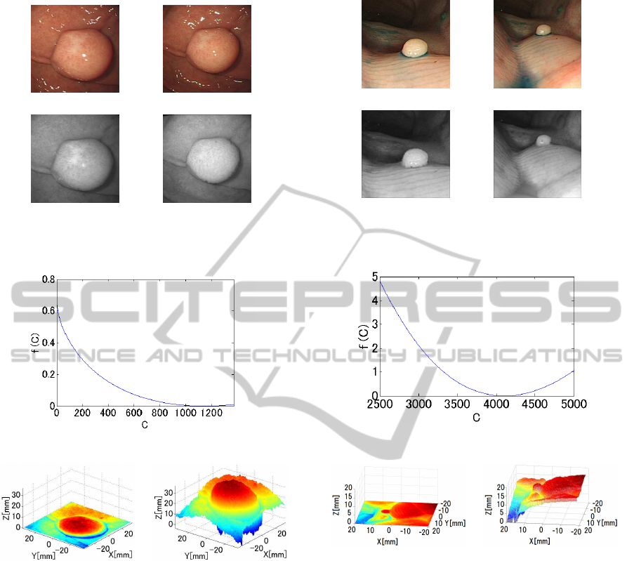
The two endoscope images are shown in Fig.13(a)
and (b). The generated Lambertian images are shown
in Fig.13(c) and (d), respectively.
The objective function, f(C), is shown in Fig.14.
The result from the VBW model is shown
in Fig.15(a) and the modified result is shown in
Fig.15(b).
The estimated value of the reflectance parameter,
C, was 1141. The difference in depth, Z, at the local
maximum point was 1 [mm] for the camera move-
ment Z
dif f
between two images. In Fig.13(c)(d),
specularities were removed compared to Fig.13(a)(b).
The converted images are gray scale with the appear-
ance of uniform reflectance. Fig.15(b) gives a larger
depth range than Fig.15(a). This suggests depth esti-
mation is improved. The size of the polyp was 1cm
and the processing time for shape modification was 9
seconds. As it took 117 seconds for NN learning with
540 epochs, a total processing time was 126 seconds.
Although quantitative evaluation is difficult, med-
ical doctors with experience in endoscopy qualita-
tively evaluated the result to confirm its correct-
ness. Different values of the reflectance parameter,
ImprovementofRecoveringShapefromEndoscopeImagesUsingRBFNeuralNetwork
67
(a) Endoscope 1 (b) Endoscope 2
(c) Lambert 1 (d) Lambert 2
Figure 13: Endoscope Image and Generating Lambert Im-
age.
Figure 14: Objective Function f (C).
(a) Z by VBW (b) Modified Z
Figure 15: Result for Endoscope Images.
C, were estimated in different experimental environ-
ments. The absolute size of a polyp is estimated based
on the estimated value ofC. Accurate values of C lead
to accurate estimation of the size of the polyp. The
estimated polyp sizes were seen as reasonable by the
medical doctor. This qualitatively confirms that the
proposed approach is effective in real endoscopy.
Another experiment was done for the endoscope
images shown in Fig.16(a)(b). The generated gray
scale Lambertian images are shown in Fig.16(c)(d),
respectively. Here the focal length is 10mm, image
size is 5mm×5mm, pixel size is 256×256 and ∆Z was
set to be 10mm.
The graph of f (C) is shown in Fig.17. The VBW
result for Fig.16(d) is shown in Fig.18(a), while that
for the proposed approach is shown in Fig.18(b).
(a) Endoscope 1 (b) Endoscope 2
(c) Lambert 1 (d) Lambert 2
Figure 16: Endoscope Image and Generating Lambert Im-
age.
Figure 17: Objective Function f (C).
(a) Z by VBW (b) Modified Z
Figure 18: Result for Endoscope Images.
C was estimated as 4108 from Fig.17. Fig.18(b)
shows greater depth amplitude compared to Fig.18(a).
The estimated size of the polyp was about 5mm.
This corresponds to the convex and concave shape es-
timation based on a stain solution. It took 60 seconds
for NN learning with 420 epochs and a total process-
ing time was 70 seconds.
4% Gaussian noise was added to a real image
and the corresponding results are shown in Fig.19(a).
Shape was estimated from the generated Lambertian
image, shown in Fig.19(b). The corresponding results
are shown in Fig.19(c) and Fig.19(d). Here the focal
length is 10mm, image size is 5mm×5mm, pixel size
is 256×256 and ∆Z was 3mm.
In this paper, it is assumed that movement of the
endoscope is constrained to be in the depth, Z, direc-
tion only. Here, it is seen that the result is acceptable
ICPRAM2015-InternationalConferenceonPatternRecognitionApplicationsandMethods
68
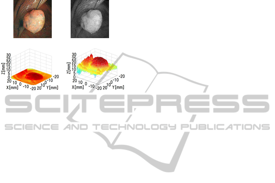
even when camera movement is in another direction,
provided rotation is minimal and the overall camera
movement is still small.
(a) Endoscope (b) Lambert
(c) Z by VBW (d) Modified Z
Figure 19: Result with Gaussian Noise.
The reflectance parameter, C, was estimated as
13244 and Fig.19(b) shows the final estimated shape.
Total of processing time was 90 seconds including 80
seconds for NN learning with 480 epochs.
The estimated size of this polyp was about 1cm.
Although Gaussian noise was added, shape recovery
remained robust.
5 CONCLUSION
This paper proposed a new approach to improve the
accuracy of absolute size and shape determination of
polyps observed in endoscope images.
An RBF-NN was used to modify surface gradi-
ent estimation based on training with data from a syn-
thesized sphere. The VBW model was used to esti-
mate a baseline shape. Modification of gradients with
the RBF-NN improved the accuracy of that baseline
shape estimation. Estimation of the reflectance pa-
rameter, C, was achieved under the assumption that
two images are acquired via small camera movement
in the depth, Z, direction. The RBF-NN is non-
parametric in that no parametric functional form has
been assumed for gradient modification. The ap-
proach was evaluated both in computer simulation
and with real endoscope images. Results confirm
that the approach improves the accuracy of recov-
ered shape to within error ranges that are practical for
polyp analysis in endoscopy.
ACKNOWLEDGEMENT
Iwahori’s research is supported by Japan Society for
the Promotion of Science (JSPS) Grant-in-Aid for
Scientific Research (C) (26330210) and Chubu Uni-
versity Grant. Woodham’s research is supported
by the Natural Sciences and Engineering Research
Council (NSERC). The authors would like to thank
Kodai Inaba for his experimental help and the related
member for useful discussions in this paper.
REFERENCES
Benton, S. H. (1977). The Hamilton- Jacobi Equation: A
Global Approach. In Academic Press, Volume 131.
Ding, Y., Iwahori, Y., Nakamura, T., He, L., Woodham,
R. J., and Itoh, H. (2010). Shape Recovery of Color
Textured Object Using Fast Marching Method via
Self-Caribration. In EUVIP 2010, pp. 92-96.
Ding, Y., Iwahori, Y., Nakamura, T., Woodham, R. J., He,
L., and Itoh, H. (2009). Self-calibration and Image
Rendering Using RBF Neural Network. In KES 2009,
Volume 5712, pp. 705-712.
Horn, B. K. P. (1975). Obtaining Shape from Shading In-
formation. In The Psychology of Computer Vision,
Winston, P. H. (Ed.), Mc Graw- Hill, pp. 115-155. Mc
Graw- Hill.
Iwahori, Y., Iwai, K., Woodham, R. J., Kawanaka, H.,
Fukui, S., and Kasugai, K. (2010). Extending Fast
Marching Method under Point Light Source Illumi-
nation and Perspective Projection. In ICPR2010, pp.
1650-1653.
Iwahori, Y., Shibata, K., Kawanaka, H., Funahashi, K.,
Woodham, R. J., and Adachi, Y. (2014). Shape from
SEM Image Using Fast Marching Method and Inten-
sity Modification by Neural Network. In Recent Ad-
vances in Knowledge-based Paradigms and Applica-
tions, Advances in Intelligent Systems and Computing
234, Springer, Chapter 5, pp.73-86.
Iwahori, Y., Sugie, H., and Ishii, N. (1990). Reconstructing
Shape from Shading Images under Point Light Source
Illumination. In ICPR 1990, Vol.1, pp. 83-87.
Iwahori, Y., Woodham, R. J., Ozaki, M., Tanaka, H., and
Ishii, N. (1997). Neural Network based Photomet-
ric Stereo with a Nearby Rotational Moving Light
Source. In IEICE Trans. Info. and Syst., Vol. E80-D,
No. 9, pp. 948-957.
Kimmel, R. and Sethian, J. A. (2001). Optimal Algorithm
for Shape from Shading and Path Planning. In Jour-
nal of Mathematical Imaging and Vision (JMIV) 2001,
Vol. 14, No. 3, pp. 237-244.
Mourgues, F., Devernay, F., and Coste-Maniere, E. (2001).
3D reconstruction of the operating field for image
overlay in 3D-endoscopic surgery. In Proceedings of
the IEEE and ACM International Symposium on Aug-
mented Reality (ISAR), pp. 191-192.
ImprovementofRecoveringShapefromEndoscopeImagesUsingRBFNeuralNetwork
69

Nakatani, H., Abe, K., Miyakawa, A., and Terakawa, S.
(2007). Three-dimensional measuremen endoscope
system with virtual rulers. In Journal of Biomedical
Optics, 12(5):051803.
Neog, D. R., Iwahori, Y., Bhuyan, M. K., Woodham, R. J.,
and Kasugai, K. (2011). Shape from an Endoscope
Image Using Extended Fast Marching Method. In
Proc. of IICAI-11, pp. 1006-1015.
Prados, E. and Faugeras, O. (2003). A mathematical and
algorithmic study of the Lambertian SFS problem for
orthographic and pinhole cameras. In Technical Re-
port 5005, INRIA 2003.
Prados, E. and Faugeras, O. (2005). Shape From Shading:
a well-posed problem? In CVPR 2005, pp. 870-877.
Prados, E. and Faugeras, O. D. (2004). Unifying Ap-
proaches and Removing Unrealistic Assumptions in
Shape from Shading: Mathematics Can Help. In
ECCV04.
Sethian, J. A. (1996). A Fast Marching Level Set Method
for Monotonically Advancing Fronts. In Proceedings
of the National Academy of Sciences of the United
States of America (PNAS U.S.), Vol. 93, No. 4, pp.
1591-1593.
Shimasaki, Y., Iwahori, Y., Neog, D. R., Woodham, R. J.,
and Bhuyan, M. K. (2013). Generating Lambertian
Image with Uniform Reflectance for Endoscope Im-
age. In IWAIT2013, 1C-2 (Computer Vision 1), pp.
60-65.
Tatematsu, K., Iwahori, Y., Nakamura, T., Fukui, S., Wood-
ham, R. J., and Kasugai, K. (2013). Shape from En-
doscope Image based on Photometric and Geometric
Constraints. In KES 2013, Procedia Computer Sci-
ence, Elsevier, Vol.22, pp. 1285-1293.
Thormaehlen, T., Broszio, H., and Meier, P. N. (2001).
Three-Dimensional Endoscopy. In Falk Symposium,
pp. 199-212.
Vogel, O., Breuß, M., and Weickert, J. (2007). A Di-
rect Numerical Approach to Perspective Shape-from-
Shading. In Vision Modeling and Visualiz-ation(VMV)
2007, pp. 91-100.
Yuen, S. Y., Tsui, Y. Y., and Chow, C. K. (2007). A fast
marching formulation of perspective shape from shad-
ing under frontal illumination. In Pattern Recognition
Letters, Vol. 28, No.7, pp. 806-824.
ICPRAM2015-InternationalConferenceonPatternRecognitionApplicationsandMethods
70
