Unconstrained Speech Segmentation using Deep Neural Networks

Van Zyl van Vuuren

, Louis ten Bosch

and Thomas Niesler

Department of Electrical and Electronic Engineering, University of Stellenbosch, Stellenbosch, South Africa

Department of Linguistics, Radboud University, Nijmegen, The Netherlands

Keywords:

Unconstrained Automatic Speech Segmentation, Deep Neural Networks, Generative Pre-training.

Abstract:

We propose a method for improving the unconstrained segmentation of speech into phoneme-like units using

deep neural networks. The proposed approach is not dependent on acoustic models or forced alignment, but

operates using the acoustic features directly. Previous solutions of this type were plagued by the tendency to

hypothesise additional incorrect phoneme boundaries near the phoneme transitions. We show that the appli-

cation of deep neural networks is able to reduce this over-segmentation substantially, and achieve improved

segmentation accuracies. Furthermore, we ﬁnd that generative pre-training offers an additional beneﬁt.

1 INTRODUCTION

Speech can be segmented into phonemes manually

by phonetic specialists, but this is known to be te-

dious, expensive and subjective. The use of accu-

rate and reliable automatic segmentation algorithms

is a desirable alternative. Especially when little or no

transcribed phonetic material is available, such algo-

rithms can facilitate the development of pronunciation

dictionaries, and can be used to obtain suitable boot-

strapping acoustic training data, thereby substantially

accelerating the development of automatic speech

recognition (ASR) systems. Automatic segmentation

algorithms are also useful outside ASR, such as for

the study of pronunciation variation, the development

of coherent large-scale dictionaries, and in text-to-

speech (TTS) applications (Sharma and Mammone,

1996; Wang et al., 2003; Adell et al., 2005).

A distinction can be made between segmenta-

tion approaches that require phone or orthographic

transcripts, and those that do not. These two ap-

proaches are often referred to as constrained and un-

constrained respectively (Keri and Prahallad, 2010).

Constrained speech segmentation algorithms are

usually based on a forced alignment between phone-

based hidden Markov models (HMMs) and the acous-

tic feature (Adell et al., 2005; Keri and Prahallad,

2010; Hoffmann and Pﬁster, 2010). In a severely

under-resourced setting, it may not be possible to ob-

tain suitable phone models. Indeed, the phone inven-

tory itself may not yet be fully known.

Unconstrained speech segmentation algorithms

detect segment boundaries using only the acoustic

features. Because this approach does not require

acoustic models, it can for example be applied in sit-

uations where the phone inventory has not yet been

established. Popular past approaches to this problem

are based on ﬁnding peaks in vector distance func-

tions that respond to the dynamics of the acoustic fea-

tures (Aversano et al., 2001; Sarkar and Sreenivas,

2005; Estevan et al., 2007; ten Bosch and Cranen,

2007; R

anen et al., 2011). The focus of this paper

is speciﬁcally on unconstrained speech segmentation.

Artiﬁcial neural networks (ANNs) have been ap-

plied to both constrained and unconstrained speech

segmentation. In the former case, use is usually made

of hybrid HMM/ANN systems in which multilayer

perceptrons (MLPs) act either as phone probability

estimators (Finster, 1992; Malfrere et al., 1998), or

are used to detect phoneme transitions in order to

reﬁne the boundaries produced by an HMM align-

ment (Toledano, 2000; Lee, 2006). In the latter case,

the ANN’s are trained to estimate a local score, which

is a value that indicates rapid changes in the features

extracted from the audio signal, and therefore gives

an indication of when a phoneme boundary is likely

to be present (Suh and Lee, 1996; Keri and Prahal-

lad, 2010). Maxima in the local score that are above

a certain threshold are taken to correspond to a hy-

pothesised segment boundary. This family of algo-

rithms can deliver excellent performance but also suf-

fers from the insertion of surplus boundaries (over-

segmentation). These are due to clusters of maxima

in the local score, not all of which correspond to true

248

Zyl van Vuuren V., ten Bosch L. and Niesler T..

Unconstrained Speech Segmentation using Deep Neural Networks.

DOI: 10.5220/0005201802480254

In Proceedings of the International Conference on Pattern Recognition Applications and Methods (ICPRAM-2015), pages 248-254

ISBN: 978-989-758-076-5

 2015 SCITEPRESS (Science and Technology Publications, Lda.)

boundaries. Recently, we have addressed this by em-

bedding an ANN local score estimator within a dy-

namic programming (DP) framework, and were able

to show reduced over-segmentation and improved

performance (van Vuuren et al., 2013). In the cur-

rent paper we build on this work by employing deep

neural network architectures as local score estimators.

The remainder of this paper is structured as fol-

lows. Sections 2 and 3 describe the application of

deep belief networks to the unconstrained segmenta-

tion problem, Section 4 describes the way in which

we assess the accuracy of competing systems, and

Sections 5 and 6 respectively describe the experimen-

tal set-up and results. Finally, Section 7 concludes.

2 RESTRICTED BOLTZMANN

MACHINES

Restricted Boltzmann machines (RBMs) have proved

to be useful building blocks in the creation of deep

neural architectures, and have recently achieved high

accuracies in phone classiﬁcation experiments (Mo-

hamed et al., 2012). We hoped to emulate this success

for the unconstrained speech segmentation task by us-

ing RBMs to achieve a more accurate local score.

An RBM is an energy-based stochastic generative

model that can learn a probability distribution from

observations by training the parameters of an undi-

rected bipartite graph, also known as a Markov ran-

dom ﬁeld (MRF) (Fischer and Igel, 2012). The vis-

ible nodes v = (v

, ..., v

) and hidden nodes (latent

variables) h = (h

, ..., h

) are illustrated in Figure 1,

where each node represents a random variable.

Figure 1: A restricted Boltzmann machine (RBM).

Each node has an associated real-valued bias in-

dicated by b

and c

for the ith visible and jth hidden

node respectively. Furthermore, each undirected con-

nection (edge) between a visible node v

∈ {1, ..., m}

and hidden node h

∈{1, ..., n}has an associated real-

valued weight w

i j

. The joint probability distribution

over visible and hidden nodes is the Boltzmann dis-

tribution (Bishop et al., 2006), and is given by Equa-

tion 1,

p(v, h) =

−E(v, h)

(1)

where Z is the partition function given by Equation 2.

Z =

∑

v, h

−E(v, h)

(2)

Associated with each conﬁguration of values for

the visible v and hidden h nodes of the RBM is a

scalar value E(v, h) called the energy as given by

Equation 3.

E(v, h) = −

∑

i=1

∑

j=1

i j

−

∑

i=1

−

∑

j=1

(3)

Binary RBMs have binary stochastic nodes for

which the visible and hidden nodes have associated

binary values, i.e. (v, h) ∈ {0, 1}

m+n

. Furthermore,

the probability of a 1 being associated with a visi-

ble or hidden node, given the hidden or visible vec-

tors respectively, can be shown to be a sigmoid func-

tion. To increase the probability of an observed or

training vector the weights are adjusted by gradient

ascent in order to maximise the log-likelihood of the

training sample. Since this is exponentially computa-

tionally expensive, an approximate training procedure

known as contrastive divergence (CD) is used instead

of the exact maximum likelihood learning (Bengio,

2009; Krizhevsky and Hinton, 2009; Fischer and Igel,

2012). CD employs Gibbs sampling to sample from

the model’s distribution. The resulting weight update

is given by Equation 4, where ε is the learning rate

and v

is the k

Gibbs sample. The update equation

for the biases is similar.

∆w

i j

= ε(p(h

= 1|v

−p(h

= 1|v

)

(4)

In the literature it is common to use 1 step CD (Er-

han et al., 2010), and this approach was followed in

our experiments.

Because the input will be real-valued, the visible

nodes of the RBM at the bottom of the stack of RBMs

will be modelled as Gaussian instead of binary. An

RBM with Gaussian visible nodes and binary hidden

nodes is referred to as a Gaussian-Bernoulli RBM

(GBRBM), and has the energy function shown in

Equation 5 (Krizhevsky and Hinton, 2009), where σ

is the standard deviation of the i

visible Gaussian

variable.

E(v, h) =

∑

i=1

−b

)

2σ

−

∑

j=1

−

∑

i=1

∑

j=1

i j

(5)

UnconstrainedSpeechSegmentationusingDeepNeuralNetworks

249

To simplify learning, some authors (Cho et al.,

2011) advise the use of a ﬁxed variance, commonly

= 1. The conditional probability for the visible

nodes given the hidden nodes is then given by Equa-

tion 6,

p(v

= v|h) = N



+ σ

∑

i j

, 1

(6)

where N (·|µ, σ

) is a Gaussian distribution with

mean µ and variance σ

. Another simpliﬁcation is to

use the means (µ

) of the visible nodes (Equation 6)

as the samples instead of sampling from the Gaus-

sian distribution during Gibbs sampling. This is done

because the standard deviations are not updated and

therefore samples from the Gaussian distribution will

be either dominated by noise or are only slightly af-

fected by the standard deviation. These restrictions

were applied in the experiments that follow, and there-

fore all the features in the training data were prepro-

cessed to have zero mean and unit variance before

training the GBRBM. In this way the contrastive di-

vergence algorithm can remain unchanged.

3 PRE-TRAINING OF DEEP

NETWORKS

To generatively pre-train a deep network, RBMs are

stacked in layers. The ﬁrst RBM is a GBRBM trained

to generate the input data. After this, the proba-

bility of activation for the hidden nodes, generated

from the training data, is used as the training data for

next RBM layer. This procedure is known as greedy

layer-wise learning (Hinton et al., 2006; Bengio et al.,

2007). As the RBMs are stacked, more abstract fea-

tures are detected by the higher RBMs. Finally a layer

of neurons corresponding to the labels of the classiﬁ-

cation problem is added to the top of the the network.

The parameters of the network can then be ﬁne-tuned

by backpropagation. We will conduct experiments

both with and without generative pre-training of the

networks in order to establish its beneﬁts for the un-

constrained speech segmentation task.

4 ASSESSMENT OF

SEGMENTATION ACCURACY

The R-value is a scalar value between 0 and 1 that

has been proposed for the assessment of segmentation

accuracy (R

anen et al., 2009). Equations 7 and 8

deﬁne two quantities known as the hit rate (HR) and

over-segmentation (OS) respectively in terms of the

number of hits (N

hit

), the number of hypothesised

boundaries (N

), and the number of reference bound-

aries (N

re f

) in an utterance. The number of hits is the

number of hypothesised boundaries within 20ms of a

true boundary.

HR =

hit

re f

(7)

OS =

re f

−1 (8)

The R-value is deﬁned as the average of two dis-

tances r

and r

which are themselves deﬁned on a

plane whose axes are HR and OS. The distances r

and r

are determined by using Equations 9 and 10

respectively, and subsequently the R-value by Equa-

tion 11.

(1 −HR)

+ OS

(9)

−OS + HR −1

√

(10)

R = 1 −

abs(r

) + abs(r

)

(11)

The larger r

or r

, the smaller the R-value will

become. Hence, the larger the R-value, the better

the segmentation performance. Informal testing re-

vealed that when the number of hypothesised bound-

aries becomes substantially more than the number of

true phoneme boundaries, it is likely that the neural

network is overﬁtting. The R-value strongly penalises

over-segmentation, and is therefore effective at com-

bating overﬁtting when using early stopping during

training, as described later in Section 5.3. Other per-

formance measures found in the literature do not ex-

plicitly penalise over-segmentation.

5 EXPERIMENTAL SET-UP

5.1 Data

Our experimental evaluations are based on the TIMIT

database (Fisher et al., 1986), which has also been

employed by several other authors for the evalu-

ation of unconstrained speech segmentation algo-

rithms (Aversano et al., 2001; Sarkar and Sreenivas,

2005; Estevan et al., 2007; Keri and Prahallad, 2010;

anen et al., 2011). The TIMIT data offers a pho-

netic segmentation (i.e. the locations of phone bound-

aries) that has been produced by human phonetic ex-

perts. Such a carefully prepared manual segmentation

is not found in other, more recent, speech databases.

ICPRAM2015-InternationalConferenceonPatternRecognitionApplicationsandMethods

250

The standard TIMIT 462-speaker training set will

be used to train the segmentation algorithms. The

development set consists of 50 speakers drawn from

the full 168-speaker test set, and is used to optimise

high-level parameters of the algorithms (Halberstadt,

1998). The standard TIMIT 24-speaker core test set is

used exclusively for ﬁnal testing. There is no speaker

overlap between any of these three sets.

In all experiments, a frame length of 10ms with

a frame skip of 5ms was used during feature extrac-

tion. Each frame of speech was represented by a 39-

dimensional feature vector consisting of 12 MFCCs,

log energy, and appended ﬁrst and second derivatives.

5.2 Baseline Systems

For purposes of comparison, two unconstrained seg-

mentation systems were included as baselines for our

proposed approach. These baseline systems have

been described previously by (Keri and Prahallad,

2010) and by (van Vuuren et al., 2013).

5.2.1 MLP-based Segmentation

A multi-layer perceptron (MLP) can be used to com-

pute a local score on the basis of a group of consec-

utive feature vectors by training an output neuron to

produce a 1 when the evidence in the input feature

vectors supports the presence of a boundary, and a

value of 0 when the evidence supports the absence of

a boundary. This approach has been shown by (Keri

and Prahallad, 2010) to lead to state-of-the-art perfor-

mance. This system has therefore been included as a

baseline for our experiments.

A segment boundary is hypothesised at the frame

at which the local score is at a maximum within a

search region, as demonstrated by Equation 12.

[

] = argmax

t∈{S

...E

}

{LS(i

)} (12)

Here i

is the i

frame, S

and E

are the start and

end of the search region respectively, LS(i

) is the lo-

cal score at frame i

, and B

is the hypothesised seg-

ment boundary. The search region is deﬁned as an

interval within which the local score exceeds a value

of 0.5.

As proposed by (Keri and Prahallad, 2010), our

baseline MLP-based segmentation system used a net-

work with single hidden layer and 30 hidden neurons.

Training data consisted of feature vector groups lo-

cated around phoneme boundaries in the TIMIT train-

ing set and feature vector groups midway between

two boundaries. The network was trained using back-

propagation without pre-training, with groups of 11

feature vectors centred about the point of interest.

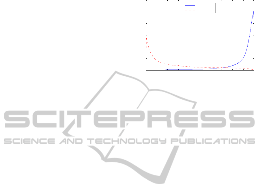
0 0.1 0.2 0.3 0.4 0.5 0.6 0.7 0.8 0.9 1

0.005

0.01

0.015

0.02

0.025

0.03

Local score

Probability

Boundary

No boundary

Figure 2: Probability distribution of MLP-based local score

values at, and away from, phoneme boundaries, estimated

from TIMIT.

Figure 2 shows the distribution of the local score

values computed on the TIMIT corpus by the result-

ing MLP. The limited overlap of these two distribu-

tions indicates that the local score can achieve good

discrimination between locations at which a bound-

ary is present, and location where it is not.

5.2.2 Dynamic Programming

The local score can be embedded in a dynamic pro-

gramming (DP) framework that includes an explicit

probabilistic model for the length of a segment. The

segmentation of a speech utterance is then formulated

as a Markov model, where each frame corresponds

to a state. The transition probabilities correspond

to the probability of the corresponding hypothesised

segment length, as established from a corpus such as

TIMIT and shown in Figure 3. The Markov emis-

sion probabilities are calculated from the distribution

of the local score values LS(i

), which were shown in

Figure 2.

Using these distributions, the probability of a

boundary given the local score at a particular frame

can be calculated and this serves as the basis of the DP

search. We have shown recently that this embedding

of a MLP-based local score in a DP framework can re-

duce the insertion incorrect boundaries when the local

score exhibits multiple closely-spaced maxima (van

Vuuren et al., 2013). We have therefore included such

a system as a second baseline for our experiments.

5.3 RBM-based Systems

All RBM-based systems used in our experiments have

logistic sigmoid neurons, since sigmoid functions are

also used to sample values from an RBM. We will

consider networks with between 1 and 5 hidden lay-

ers, with each hidden layer having the same number

UnconstrainedSpeechSegmentationusingDeepNeuralNetworks

251

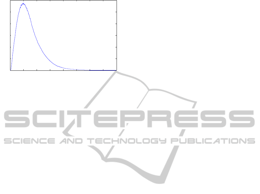
0 50 100 150 200 250 300 350 400

0.002

0.004

0.006

0.008

0.01

0.012

Probability

Segment length (ms)

Figure 3: Probability distribution of phoneme lengths in the

TIMIT training set.

of neurons (256, 512 or 1024). For each network ar-

chitecture, a network is prepared with and without

pre-training. The subsequent supervised training by

backpropagation employs early stopping to ﬁnd the

best performing network on the development set, af-

ter which the network’s performance was tested on

the TIMIT core test set.

Early stopping is a technique used to avoid

overﬁtting during supervised training of neural net-

works (Erhan et al., 2010). After each training epoch

the network’s development set performance is com-

pared to the previous epoch’s performance. When the

performance deteriorates, the learning rate is halved.

Training then continues from the previous epoch’s

weight values. We found that the networks’s perfor-

mance tends to alternate slightly between epochs, al-

though improving in the longer term. For this reason

we chose to halve the learning rate only when the per-

formance drops consistently over 5 trial epochs.

For generative pre-training each RBM was sub-

jected to 50 training epochs, i.e. 50 epochs of un-

supervised training per layer of the DBN, at a learn-

ing rate of 0.005 for the Gaussian Bernoulli RBM

and 0.05 for the binary RBMs, and with a momen-

tum of 0.9. These values were chosen to be similar

to those used to train RBM-based acoustic models for

phone classiﬁcation (Mohamed et al., 2012). Early

stop training starts with a learning rate of 0.1 and mo-

mentum of 0.9, and continues until the learning rate is

smaller than 0.01. Stochastic gradient descent and un-

supervised pre-training used mini-batches consisting

of 128 training samples.

An input vector to the neural network consisted

of the features associated with 11 consecutive frames

centred on the test frame. Since the feature vector

extracted from each frame was 39-dimensional, each

input vector had a total of 429 components.

6 EXPERIMENTAL RESULTS

Every network architecture was subjected to three

early stop training sessions, from which a mean per-

formance was calculated. This average is taken to in-

dicate typical performance. Figure 4 shows this per-

formance on the TIMIT core test set for 256, 512, and

1024 hidden neurons per hidden layer.

When the number of hidden layers is increased

from 1 to 2, there is in all cases a notable performance

improvement. However, when 3 or more hidden lay-

ers are used, further gains are not reliably achieved.

There is gradual improvement in performance as the

number of neurons per hidden layer is increased.

The core test set performance of the networks with

best performance on the development set, with and

without pre-training are shown in Table 1. The net-

works with and without pre-training contained 5 and

3 hidden layers respectively, both with 1024 neurons

per layer (Figure 4). The performance of the pre-

trained network when embedded in the DP algorithm

as described in Section 5.2.2 is also shown.

Hypothesised boundaries falling outside a 20ms

region around the true phoneme boundaries are re-

garded as insertions, and missed phoneme bound-

aries as deletions. The average percentage insertions

and deletions per reference phoneme boundary are in-

cluded in the table. Both deep networks achieve sub-

stantial improvements in segmentation performance.

Best performance is achieved when pre-training is ap-

plied. It is interesting to see that the incorporation

of dynamic programming leads to deteriorated per-

formance in our DNN experiments. Since the chief

motivation for the dynamic programming framework

was to reduce over-segmentation, this indicates that

the local scores estimated by the deep networks are

less prone to these insertion errors, and therefore the

incorporation of DP is unnecessary and even counter-

productive.

7 DISCUSSION AND

CONCLUSION

Our experiments show that a deep neural network is

able to provide a substantially better local score for

use in unconstrained speech segmentation than previ-

ously proposed alternatives. Pre-training provides a

performance beneﬁt, as does a larger number of neu-

rons per hidden layer. Furthermore, the local scores

estimated by deep networks appear to reduce the ten-

dency to over-segment that has been associated with

this class of algorithms in the past. Other means of re-

ducing over-segmentation, such as the introduction of

ICPRAM2015-InternationalConferenceonPatternRecognitionApplicationsandMethods

252

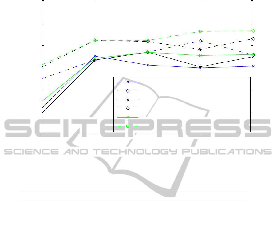
1 2 3 4 5

0.865

0.87

0.875

0.88

0.885

0.89

0.895

Hidden layers

R−value

256 neurons with no pre−training

256 neurons with pre−training

512 neurons with no pre−training

512 neurons with pre−training

1024 neurons with no pre−training

1024 neurons with pre−training

Figure 4: Segmentation performance on the TIMIT core test set for networks with 256, 512, and 1024 hidden neurons per

layer, and with between 1 and 5 hidden layers.

Table 1: Comparison of segmentation performance, measured on the TIMIT core test set, of systems with best performance

on the development set.

System

Ins(%) Del(%) R-value

MLP benchmark from (Keri and Prahallad, 2010) 12.74 17.00 0.857

MLP with DP benchmark from (van Vuuren et al., 2013) 13.06 15.72 0.863

DNN without pre-training 11.17 12.73 0.887

DNN with pre-training 10.14 12.66 0.891

DNN with DP and pre-training 13.12 14.05 0.868

probabilistic models for segment length and dynamic

programming, therefore no longer lead to any perfor-

mance beneﬁt. This simpliﬁes the segmentation algo-

rithm.

In the future we plan to investigate whether the

performance beneﬁt of our proposed algorithm per-

sists when applied to data substantially different from

the TIMIT training material. We are particularly in-

terested to know the behaviour of unconstrained seg-

mentation algorithms trained on TIMIT but applied

to entirely different languages. Eventually, we would

like to determine whether such cross-domain segmen-

tation can be used to facilitate the development of

ASR systems for under-resourced languages.

ACKNOWLEDGEMENTS

This research was supported by the National Research

Foundation of South Africa under grant UID 71926.

Opinions expressed and conclusions arrived at are

those of the authors and are not necessarily to be at-

tributed to the NRF.

REFERENCES

Adell, J., Bonafonte, A., Gomez, J., and Castro, M. (2005).

Comparative study of automatic phone segmentation

methods for TTS. In Proceedings of the IEEE Inter-

national Conference on Acoustics, Speech, and Signal

Processing (ICASSP).

Aversano, G., Esposito, A., Esposito, A., and Marinaro, M.

(2001). A new text-independent method for phoneme

UnconstrainedSpeechSegmentationusingDeepNeuralNetworks

253

segmentation. In Proceedings of the 44th IEEE Mid-

west Symposium on Circuits and Systems.

Bengio, Y. (2009). Learning deep architectures for AI.

Foundations and Trends in Machine Learning, 2(1):1–

127.

Bengio, Y., Lamblin, P., Popovici, D., and Larochelle, H.

(2007). Greedy layer-wise training of deep networks.

Advances in neural information processing systems,

19:153.

Bishop, C. M. et al. (2006). Pattern recognition and ma-

chine learning, volume 1. Springer.

Cho, K. et al. (2011). Improved learning algorithms for re-

stricted Boltzmann machines. Master’s thesis, School

of science, Aalto University.

Erhan, D., Bengio, Y., Courville, A., Manzagol, P.-A., Vin-

cent, P., and Bengio, S. (2010). Why does unsuper-

vised pre-training help deep learning? The Journal of

Machine Learning Research, 11:625–660.

Estevan, Y. P., Wan, V., and Scharenborg, O. (2007). Find-

ing maximum margin segments in speech. In Proceed-

ings of the IEEE International Conference on Acous-

tics, Speech, and Signal Processing (ICASSP).

Finster, H. (1992). Automatic speech segmentation us-

ing neural network and phonetic transcription. In

Proceedings of the International Joint Conference on

Neural Networks (IJCNN).

Fischer, A. and Igel, C. (2012). An introduction to restricted

Boltzmann machines. In Progress in Pattern Recogni-

tion, Image Analysis, Computer Vision, and Applica-

tions, pages 14–36. Springer.

Fisher, W. M., Doddington, G. R., and Goudie-Marshall,

K. M. (1986). The DARPA speech recognition re-

search database: speciﬁcations and status. In Proceed-

ings of the DARPA Workshop on Speech Recognition.

Halberstadt, A. K. (1998). Heterogeneous Acoustic Mea-

surements and Multiple Classiﬁers for Speech Recog-

nition. PhD thesis, Massachusetts Institute of Tech-

nology, MIT.

Hinton, G. E., Osindero, S., and Teh, Y.-W. (2006). A fast

learning algorithm for deep belief nets. Neural com-

putation, 18(7):1527–1554.

Hoffmann, S. and Pﬁster, B. (2010). Fully automatic seg-

mentation for prosodic speech corpora. In Proceed-

ings of Interspeech.

Keri, V. and Prahallad, K. (2010). A comparative study

of constrained and unconstrained approaches for seg-

mentation of speech signal. In Proceedings of the In-

ternational Conference on Spoken Language Process-

ing (ICSLP).

Krizhevsky, A. and Hinton, G. (2009). Learning multiple

layers of features from tiny images. Master’s the-

sis, Department of Computer Science, University of

Toronto.

Lee, K.-S. (2006). MLP-based phone boundary reﬁning for

a TTS database. IEEE Transactions on Audio, Speech

and Language Processing, 14(3):981–989.

Malfrere, F., Deroo, O., and Dutoit, T. (1998). Pho-

netic alignment : Speech synthesis based vs. hybrid

HMM/ANN. In Proceedings of the International Con-

ference on Spoken Language Processing (ICSLP).

Mohamed, A.-r., Dahl, G. E., and Hinton, G. (2012).

Acoustic modeling using deep belief networks. IEEE

Transactions on Audio, Speech, and Language Pro-

cessing, 20(1):14–22.

anen, O., Laine, U., and Altosaar, T. (2011). Blind seg-

mentation of speech using non-linear ﬁltering meth-

ods. Speech Technologies, pages 105–124.

anen, O. J., Laine, U. K., and Altosaar, T. (2009). An

improved speech segmentation quality measure: the

R-value. In Proceedings of Interspeech).

Sarkar, A. and Sreenivas, T. (2005). Automatic speech seg-

mentation using average level crossing rate informa-

tion. In Proceedings of the IEEE International Con-

ference on Acoustics, Speech, and Signal Processing

(ICASSP).

Sharma, M. and Mammone, R. (1996). ‘Blind’ speech seg-

mentation: automatic segmentation of speech without

linguistic knowledge. In Proceedings of the Fourth In-

ternational Conference on Spoken Language Process-

ing (ICSLP).

Suh, Y. and Lee, Y. (1996). Phoneme segmentation of con-

tinuous speech using multi-layer perceptron. In Pro-

ceedings of the Fourth International Conference on

Spoken Language (ICSLP).

ten Bosch, L. and Cranen, B. (2007). A computational

model for unsupervised word discovery. In Proceed-

ings of Interspeech.

Toledano, D. (2000). Neural network boundary reﬁning for

automatic speech segmentation. In Proceedings of the

IEEE International Conference on Acoustics, Speech,

and Signal Processing (ICASSP).

van Vuuren, V. Z., ten Bosch, L., and Niesler, T. (2013). A

dynamic programming framework for neural network-

based automatic speech segmentation. In Proceedings

of Interspeech.

Wang, D., Lu, L., and Zhang, H.-J. (2003). Speech segmen-

tation without speech recognition. In Proceedings of

theInternational Conference on Multimedia and Expo,

ICME.

ICPRAM2015-InternationalConferenceonPatternRecognitionApplicationsandMethods

254