
Meshing Meristems
An Iterative Mesh Optimization Method for Modeling Plant Tissue at Cell
Resolution
Guillaume Cerutti and Christophe Godin
INRIA, Virtual Plants INRIA Team, Montpellier, France
Keywords:
Mesh Optimization, Shoot Apical Meristem, Deformable Models, Cell Reconstruction, Morphogenesis.
Abstract:
We address in this paper the problem of reconstructing a mesh representation of plant cells in a complex,
multi-layered tissue structure, based on segmented images obtained from confocal microscopy of shoot apical
meristem of model plant Arabidopsis thaliana. The construction of such mesh structures for plant tissues is
currently a missing step in the existing image analysis pipelines. We propose a method for optimizing the
surface triangular meshes representing the tissue simultaneously along several criteria, based on an initial
low-quality mesh. The mesh geometry is deformed by iteratively minimizing an energy functional defined
over this discrete surface representation. This optimization results in a light discrete representation of the
cell surfaces that enables fast visualization, and quantitative analysis, and gives way to in silico physical and
mechanical simulations on real-world data. We provide a framework for evaluating the quality of the cell
tissue reconstruction, that underlines the ability of our method to fit multiple optimization criteria.
1 INTRODUCTION
The spectacular development of 3-dimensional mi-
croscopy imaging techniques over the past few years
has opened a brand new field of experimental investi-
gation for developmental biology. The huge amounts
of data produced require the development of complete
software pipelines to process automatically the image
sequences capturing the living tissues. The automatic
segmentation of cells and the tracking of cell lineages
over time allows to quantify tissue growth, cell defor-
mation and gene expression patterns.
However, segmented images constitute massive
objects, and lighter and more versatile data structures
that represent the shape of the cells are preferable to
the raw voxel information. Triangular meshes are
a compressed representation that make visualization
easier and various computations on surfaces and vol-
umes much more efficient. It is also a necessary ob-
ject for a great deal of physical simulations, notably
those based on finite elements methods. We consider
then the problem of converting a 3-dimensional image
stack of segmented cell tissue into a triangular mesh
representing the surfaces the cells.
Our work is focused on images of shoot apical
meristems (SAM) of Arabidopsis thaliana acquired
by confocal laser scanning microscopy (CLSM) such
as the one shown in Figure 1, and segmented using
the MARS software pipeline (Fernandez et al., 2010).
SAMs constitute small niches of dividing cells where
all the aerial organs of a plant (inflorescence, leaves
or branches), originate from. The study of sequences
of cell tissue on the SAM is therefore a key step for a
better understanding of morphogenesis in plants, and
the growth of organs over time. The identification of
cells, the reconstruction of their lineages and extrac-
tion of shape and semantic features at a cellular level
are necessary steps in this analysis process.
In this context, we propose a tool to reconstruct
Figure 1: Confocal laser scanning image of an inflorescence
meristem of Arabidopsis thaliana.
23
Cerutti G. and Godin C..
Meshing Meristems - An Iterative Mesh Optimization Method for Modeling Plant Tissue at Cell Resolution.
DOI: 10.5220/0005190100230035
In Proceedings of the International Conference on Bioimaging (BIOIMAGING-2015), pages 23-35
ISBN: 978-989-758-072-7
Copyright
c
2015 SCITEPRESS (Science and Technology Publications, Lda.)

automatically the whole 3-D structure of a SAM by
a discrete representation of cell surfaces. This mesh
transforms the voluminous complex images into sim-
ple 3-D primitives, and includes topological relation-
ships between cells as well as the estimation of their
shape. In the following, we will present related work
in Section 2. The generation of meshes is presented
in Section 3 as well as the evaluation criteria we intro-
duce, and the subsequent mesh optimization process
is described in Section 4. Section 5 proposes an anal-
ysis of the results, as Section 6 draws conclusions and
potential applications.
2 RELATED WORKS
The recent progresses in microscopy imaging make it
possible to record the development of living tissues
and organisms, with a temporal frequency that offers
the novel opportunity of monitoring and modelling
the processes at work at cell level (Keller, 2013).
2.1 Cell-scale Tissue Reconstruction
The interest of cell-scale tissue imaging for develop-
mental biology is tremendous, and many works aim at
building a digital reconstruction of living cells, con-
sidering different subjects of study : capturing the
dynamics of plant shoot apical meristems (Fernan-
dez et al., 2010; Tataw et al., 2013; Chakraborty
et al., 2013) or following animal embryos during dif-
ferent development stages (Robin et al., 2011; Rizzi
and Peyrieras, 2014; Guignard et al., 2014; Michelin
et al., 2014).
Concerning the development of SAM cells
(mostly of Arabidopsis thaliana) the works ini-
tially focused on the reconstruction of the surface
(Kwiatkowska, 2004) to analyse the growth and di-
vision dynamics of the first layer of cells (L1) in the
meristem (Barbier de Reuille et al., 2005). More
recently, complete reconstructions of the dynamic
multi-layered tissue structure have emerged, based on
CLSM images, using a watershed segmentation algo-
rithm (Fernandez et al., 2010) or representing cells as
truncated ellipsoids (Chakraborty et al., 2011).
In contrast with pure image segmentation where
the output is an image of labeled voxels, some meth-
ods provide a more discrete cell reconstruction, un-
der the form of a Voronoi-like anisotropic tessellation
(Chakraborty et al., 2013) or with tools allowing the
definition of a triangular mesh on the surface of the
meristem (Barbier de Reuille et al., 2014). Such a
compact tissue reconstruction is a desirable output for
fast quantification of cell properties, interactive visu-
alization of large objects and models of tissue growth.
2.2 Mesh Generation and Optimization
A triangular mesh constitutes a discretization of a sur-
face or a volume, and a generally more compressed
view of an object, making it easier to manipulate. Dif-
ferent approaches have emerged to generate a mesh
from a 3-dimensional image, most commonly using
Marching Cubes (Lorensen and Cline, 1987) to pro-
duce a very high resolution mesh of the surfaces,
or based on triangulated sample points (Shewchuk,
1998) to represent a volume by tetrahedra.
A common problem with mesh generation meth-
ods is the lack of control on the quality of the pro-
duced mesh. To obtain a satisfying result, some op-
timization is generally needed, either on the connec-
tivity of the mesh elements (through local collapse or
split operations (Hoppe et al., 1993)) or on their shape
(Owen, 1998).
To improve the shapes of the mesh elements, a
common approach is to smooth the mesh by adjust-
ing the positions of its vertices. The most widespread
method is the Laplacian smoothing (Field, 1988),
where vertices are attracted by the barycenters of their
neighbors, and that has been used widely in other
mesh smoothing techniques (Freitag, 1997).
Another method is to consider smoothing as an
optimization problem, where the quality of the mesh
can be estimated locally, and the location of any point
updated to improve the quality of its surroundings
(Amenta et al., 1997; Freitag, 1997). In that case,
the problem can be formulated as the minimization of
an energy functional (Hoppe et al., 1993; Vidal et al.,
2012), a framework that can also be used for segmen-
tation and tracking purposes (Dufour et al., 2011).
Such approaches allow a precise definition of the
properties that should be optimized by the smoothing,
as well as the inclusion of external constraints intro-
ducing some prior knowledge, and are well suited for
domain-specific applications such as ours.
3 GENERATING TISSUE MESH
The first step towards the reconstruction of a mesh
representation of a cell tissue is the generation of its
topology. This implies that all the cells in the multi-
layered structure have to be identified to make the def-
inition of interfaces between cells possible. Based on
a confocal microscopy image stack, we perform a seg-
mentation that labels each voxel with a cell identifier,
forming closed, neighboring 3-dimensional regions
BIOIMAGING2015-InternationalConferenceonBioimaging
24
that will constitute the starting point of our mesh gen-
eration.
3.1 3-D Cell Segmentation
The method we use to segment the confocal image
sequences is based on the MARS pipeline (Fernandez
et al., 2010) and uses a seeded 3-dimensional water-
shed algorithm to extract the regions corresponding
to each cell. The accurate identification of cells relies
on the determination of seeds, but the method ensures
that the regions converge towards each other, without
any hole. This guarantees that neighborhood relation
between cells and interface surfaces are well defined
in every dimension throughout the structure.
Figure 2: View of the watershed segmentation image ob-
tained on the confocal image stack of a shoot apical meris-
tem.
The resulting segmented images are complex and
heavy objects, such as the one depicted in Figure 2.
The typical number of regions in the image may reach
3000, each of them containing roughly 20000 vox-
els. In addition to this excessive weight, the seg-
mented images inevitably present some artifacts lead-
ing to noisy boundaries, which could benefit from the
smoothing induced by a coarser discrete representa-
tion.
3.2 Tetrahedral Mesh Generation
To represent the segmented cells by a mesh structure,
our strategy consists in compute the mesh topology
using a standard method, and then improve it rela-
tively to the characteristics of our data. Among the
various possibilities for generating a mesh topology
from the segmented image data, we chose to use a
tetrahedral discretization of the whole image domain,
based on a Delaunay triangulation refinement algo-
rithm (Shewchuk, 1998). Compared to other methods
such as Marching Cubes (Lorensen and Cline, 1987)
that generate a huge number of triangles, a triangu-
lation offers the advantage of reducing drastically the
volume of information, as it produces from the start a
lighter object.
Along with many other computational geometry
algorithms, this tetrahedral mesh generation is imple-
mented in the CGAL library (CGAL, 1996), and we
used this implementation to generate our mesh topol-
ogy. The resulting object is a simplicial complex of
dimension 3, where each tetrahedron is labeled with a
cell identifier.
To convert the simplicial complex into a nested
surface mesh, we get rid of the tetrahedra and keep
only the triangular faces that are common to two tetra-
hedra with different labels. Each cell is then bounded
by a set of triangles forming a closed surface. Each
one of these triangles may be part of (at most) two
cells, as the same interface triangle will be assigned to
the boundary of the two cells it separates. The result-
ing mesh constitute an approximation of the complete
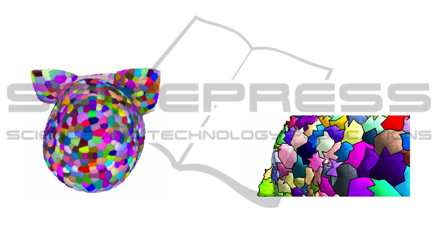
structure of the tissue, as illustrated in Figure 3.
Figure 3: Surface triangles of the mesh of shoot apical
meristem cells built from the tetrahedral mesh generated by
Delaunay refinement.
The quality of the image approximation provided
by the mesh is controlled in the CGAL implementa-
tion by a distance parameter. This value sets the up-
per bound for the distance between the mesh triangles
and the boundaries of their corresponding regions in
the image. This parameter has also a strong influence
on the complexity of the mesh, as more numerous and
smaller triangles are necessary to fit the image bound-
aries with less error. The optimization performed by
lowering this global distance constraint comes with
an exponential rise in the number of primitives used
to define the surfaces, and consequently does not op-
erate on all the desirable properties of the mesh.
3.3 Quality Criteria
The criteria we would like to see as optimal in the
mesh are multiple and not necessarily compatible.
The quality objective involves both geometrical and
biological factors that should be met with a minimal
complexity by the resulting mesh. It is then necessary
to define accurately what is a good tissue mesh, and
how it is possible to quantitatively evaluate its quality.
MeshingMeristems-AnIterativeMeshOptimizationMethodforModelingPlantTissueatCellResolution
25
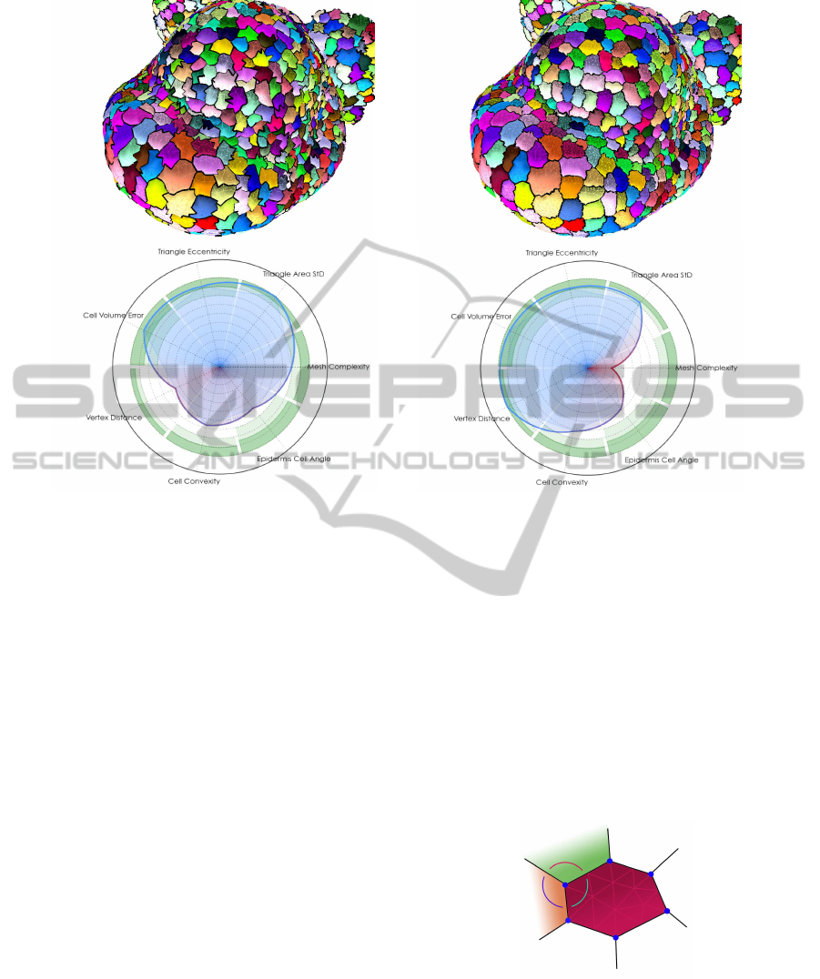
(a) (b)
Figure 4: Comparison of quality criteria measures for two meshes of the same image obtained with distance parameter values
of 2.0 voxels (a) and 1.0 voxel (b).
To perform this evaluation, we define 7 quality
criteria that account for the various objectives a cell
tissue mesh should fulfill. Those criteria concern the
precision with which the mesh fits the input data, the
consistency of the shape it defines with those expected
from SAM cells, the regularity of the triangles defin-
ing the surface, and the number of geometric elements
necessary to the representation. A thorough definition
of this criteria can be found in Section 5.
Indeed, the reconstructed cells in the final mesh,
though consisting of a simplified model, should first
correspond as precisely as possible to the cells iden-
tified in the original image, and constitute a faithful
reconstitution of the segmented voxel image S that
can be seen as a ground truth.
• Region Consistency: global measure based on
the comparison of cell volumes in the mesh and
in the original image.
• Interest Point Preservation: local measure
based on the distance of identified points in the
mesh with their matching ones in the image.
A second important aspect is the way the shape of
cells in the mesh correspond to the prior knowledge
accessible on SAM cells. The resulting mesh must
not only coincide with the computer-generated data
representing cells, but most importantly to observed
cell geometric properties, in order to become a bio-
logically plausible meristem reconstruction and make
it possible to draw conclusions from simulations (Fig-
ure 5).
• Cell Convexity: global measure based on the
convexity of the mesh cells, estimated as a vol-
ume ratio with their convex hull.
• Surface Arrangement: local measure based on
the apparent geometry of the surface cells, and the
projected angles formed by adjacent cells.
Figure 5: Example of a good quality cell with its interest
points : convex, regularly triangulated and with regular an-
gles with neighbors.
The quality of a triangular mesh is more com-
monly defined by the absence of small or eccentric
triangles. Given the goal of using the meshed meris-
tems for physical simulations, the triangles must in
any way have properties allowing the application of
BIOIMAGING2015-InternationalConferenceonBioimaging
26

finite element methods. Consequently the regularity
and homogeneity of the mesh in the shape and size of
its surface elements has to be taken into account.
• Triangle Quality: global measure based on a tri-
angle eccentricity estimation, measuring how far
a given triangle is from an equilateral one.
• Size Homogeneity: global measure based on the
standard deviation of the areas of triangles to esti-
mate how regular the mesh is.
And finally, a highly desirable property is to reach
the aforementioned objectives with as few triangles as
possible. In terms of computational cost for visualiza-
tion and feature extraction, the lighter the mesh is, the
better performance will be reached, provided that the
other criteria are fulfilled.
• Mesh Lightness: global measure based on the
number of triangles necessary to represent the sur-
face of a cell.
A simultaneous view of all these quality criteria can
be given by a spider chart, as soon as all measurement
can be aligned on the same scale (by a normalization
between 0 and 1 for instance). This results in a visual-
ization such as those presented in Figure 4 where the
overall area of the domain delimited by the values of
the different parameters has to be maximal. Any de-
fect in one of the criteria will immediately be reflected
in the visualization chart.
Applied to the surface meshes produced by the
Delaunay refinement algorithm, such quality estima-
tion highlights the complex optimization problem we
are facing. The objective being to maximize all the
criteria at the same time, improving the mesh by low-
ering the distance parameter is not satisfactory, given
the drastic loss on the lightness criterion, as it appears
strikingly in Figure 4. An acceptable solution should
be more of a compromise that tends to optimize all
quality criteria for a fixed mesh complexity.
4 MESH OPTIMIZATION
To address the problem emerging from the introduced
criteria, we choose to formulate this mesh optimiza-
tion as an energy minimization problem, in the same
spirit as (Hoppe et al., 1993). One objective being to
limit the mesh complexity, this task can be performed
on a light mesh without any change in its topology, by
working only on the mesh geometry.
4.1 Mesh Definitions
The mesh object M we consider is a boundary repre-
sentation of dimension 3, consisting of four sets of el-
ements W
0
,W
1
,W
2
,W
3
representing respectively ver-
tices, edges, triangles and cells.
The elements themselves are defined by their
boundaries in the dimension below, which can be rep-
resented by a boundary relationship B
d
at dimension
d. For instance, an edge e ∈ W
1
is defined by its
two vertex extremities B
1
(e) =
{
v
1
(e),v
2
(e)
}
,v
1
6=
v
2
∈ W
0
, a triangle t ∈ W
2
by its three edges. A cell
c ∈W
3
is the only type of element for which the num-
ber of boundary elements (triangles) is not fixed.
The boundary relation can be extended to con-
sider gaps of more than one dimension, for instance
to retrieve the vertices of a triangle; this higher di-
mension boundary relation B
n
d
links elements of di-
mension d with their boundaries at dimension d −n,
and can be defined recursively : ∀w ∈ W
d
,B
n
d
(w) =
S
u∈B
d
(w)
B
n−1
d−1
(u) (with B
1
d
= B
d
).
This first relationship gives birth to a converse re-
gion relationship R
n
d
representing, for an element of
dimension d, the elements of higher dimension for
which it constitutes a boundary:
∀w ∈ W
d
,R
n
d
(w) =
u ∈ W
d+n
(M ) | w ∈B
n
d+n
(u)
Those two symmetrical relations define two possi-
ble neighborhood relations N
+
d
and N
−
d
between ele-
ments of the same dimension, depending whether we
consider that they are connected by a higher dimen-
sion region (like two vertices linked by an edge) or by
a lower dimension boundary (like two cells sharing an
interface triangle):
N
+
d
(w) =
w
0
∈ W
d
| R
d
(w) ∩R
d
(w
0
) 6=
/
0
N
−
d
(w) =
w
0
∈ W
d
| B
d
(w) ∩B
d
(w
0
) 6=
/
0
In addition to this topological aspect, the geome-
try of the mesh is defined by the association of each
vertex v ∈ W
0
with a point in R
3
representing its po-
sition P (v) in the image referential. The definition of
P determines the shape of every higher dimension el-
ement, and plays a predominant part in the quality of
the mesh.
Using this representation, our optimization prob-
lem comes down to searching optimal positions P of
the vertices, an optimization that can be performed
without modification of the mesh topology if its ini-
tial configuration is satisfactory. Provided an initial
mesh M
(0)
=
W
0
,P
(0)
,W
1
,B
1
,W
2
,B
2
,W
3
,B
3
,
obtained for instance by Delaunay refinement, the
problem is to find the optimal mesh geometry P
∗
, as
the one that minimizes an energy functional account-
ing for the quality criteria.
4.2 Energy Formulation
Following the widespread approach concerning de-
formable models, from their first application to con-
MeshingMeristems-AnIterativeMeshOptimizationMethodforModelingPlantTissueatCellResolution
27

tour detection (Kass et al., 1988) to other commonly
used models (Chan and Vese, 2001), the energy func-
tional E that we aim at minimizing is defined as a sum
of energy terms accounting for the different criteria to
be optimized. This general combination applied to 3-
dimensional models (Dufour et al., 2011) can be writ-
ten as:
E(M ,S ) = E
image
(M ,S)+E
prior
(M )+E
regularity
(M )
There is an identity between the energy terms and
the quality criteria we defined. The image, or data
attachment, energy should be minimal when the re-
gion consistency and interest point preservation crite-
ria are optimal, and the same goes for the prior energy
and the cell convexity and surface arrangement crite-
ria, and the internal regularity energy and the triangle
quality and homogeneity criteria.
Each one of these three terms is built on local en-
ergy potentials defined on the elements of M (and the
geometry of their vertices) that estimate the validity
of the local configuration regarding the correspond-
ing criterion.
4.2.1 Image Attachment Energy
The surfaces represented by the mesh M are defined
to fit the separations between cells in the segmented
image S , so that the regions delimiting cells in both
representations superimpose as perfectly as possible.
More importance is given to special interest points
which are cell corners. These points correspond to
those where four cells intersect in S (or three cells at
the surface of the tissue) and should particularly be
preserved in the mesh for a realistic reconstruction.
Such points are very easily accessible in the topology
of M as the vertices v for which R
3
0
(v) contains four
elements (respectively three).
Both the region consistency and the interest point
preservation criteria refer to a notion of gradient mag-
nitude in the segmented image S , as separation inter-
faces are transitions leading to non-zero values of gra-
dient, and cell corners, where many transitions occur,
would correspond to local maximal values. However,
unlike a color or intensity image, the segmentation S
is a label image where the actual values do not matter,
only the transitions are to be considered.
Therefore, we approximate the gradient magni-
tude image k∇S k by considering a spherical neigh-
borhood of radius σ around each voxel and count the
number of different labels it encloses. To give more
weight to exterior object boundaries, the number is
doubled when the neighborhood intersects the exte-
rior. This function is then smoothed by a gaussian
filter of standard deviation σ to obtain a more contin-
uous value.
The energy E
gradient
associated with this bound-
ary information is defined on the positions P of the
vertices of the mesh, and should be minimal when a
vertex fits well on a cell interface. We define it sim-
ply as the opposite of the gradient magnitude, so that
high values of the gradient constitute optimal posi-
tions for the vertices of the mesh, weighted by a coef-
ficient ω
gradient
:
E
image
(M ,S) =
∑
v∈W
0
ω
gradient
E
gradient
(v,S)
=
∑
v∈W
0
−ω
gradient
k∇Sk(P (v))
(1)
4.2.2 Shape Prior Energy
The second energy term gives the possibility of in-
cluding prior knowledge on the geometry of cells or
additional external constraints. The most simple char-
acterization for a SAM cell, and the minimal con-
straint it should satisfy, is that its surface should form
a convex solid with convex planar polygonal facets,
such as examples in Figure 6.
Figure 6: Example of cells as convex solids with planar con-
vex polygonal facets.
From biological expertise, we expect cells to
present in most cases planar interfaces, and linear
edges that form convex faces, properties that should
fulfill the two cell shape criteria. They are translated
into two energy potentials defined on the vertices of
the mesh:
E
prior
(M ) =
∑
v∈W
0
ω
plan
E
plan
(v) + ω
line
E
line
(v)
(2)
The planarity energy potential E
plan
(v) simply
sums the distances of P (v) to the average planes of
all the cell interfaces it belongs to. Those planes are
estimated by averaging the normals of the triangles
composing the interface, and the distance can be com-
puted as a dot product.
The energy E
line
(v) is defined on the vertices be-
longing to at least two cell interfaces, thus part of the
contour of a cell interface. To regularize those con-
tours, we chose to sum the laplacian energies of all
the interface contours going through v, computed at
P (v).
BIOIMAGING2015-InternationalConferenceonBioimaging
28

4.2.3 Triangle Regularity Energy
The internal energy term accounts for the regularity
of the mesh, and for the optimization of the triangle
quality and size homogeneity criteria. This leads to a
definition of two energy potentials, this time defined
on triangles, but that can commonly be restricted to
the vertices of each triangle:
E
regularity
(M ) =
∑
v∈W
0
1
3
∑
t∈R
2
0
(v)
ω
qual
E
qual
(t)
+ ω
size
E
size
(t)
(3)
It is commonly accepted that a regular triangu-
lar surface mesh is composed of vertices of degree 6,
connecting 6 even equilateral triangles. The quality
energy potential E
qual
(t) defined on a triangle’s ge-
ometry
P (v) | v ∈B
2
2
(t)
should measure its eccen-
tricity, its deviation from an equilateral configuration.
Among the various possible triangle eccentricity mea-
sures (Field, 2000), we chose the sum of sinuses, that
involves no maximum operator, and has good deriv-
ability properties, while being optimal in the equilat-
eral case:
E
qual
(t) = 1 −
2
3
√
3
∑
v∈B
2
2
(t)
sin
d
P (v)
(4)
Concerning the size homogeneity potential
E
size
(t), we simply use the squared distance of the
triangle area to the average area over all the mesh.
Defined this way, this energy is of course minimal
when all the triangles have the same size.
4.3 Minimization and Evolution
The minimization of the energy functional E is per-
formed by a local optimization process, based on con-
secutive small moves of the vertices. The vertex posi-
tions P are iteratively updated to decrease the overall
value of the energy function, based on decisions made
locally on the energy potentials.
To add more control on this operation, at each it-
eration i, we force the updated position P
(i+1)
(v) of
each vertex to remain within a sphere of radius σ
v
around its current position P
(i)
(v). This limitation en-
sures that the mesh deforms smoothly and limits the
risk of fold-overs and intersections between triangles.
The motion of the vertices can be determined by
a gradient descent of the local energy potential, fol-
lowing the opposite direction of the local gradient of
E, i.e. the first order derivative of the energy with re-
spect to P , while staying inside the sphere of radius
σ
v
around P (v):
P
(i+1)
(v) = P
(i)
(v) −min
1,
σ
v
∂E
∂P
v
∂E
∂P
v
(5)
The only exception concerns cell corners, as a
matching can directly be performed between those in-
terest points in the mesh and in the image. Their opti-
mal position can therefore be known in advance, and
the iterative shifting for the vertices v of M that could
be matched to a cell corner in S will simply consist in
smoothly traveling along the trajectory between their
initial position P
(0)
(v) and their corresponding image
target point P
(S)
(v).
For the remaining vertices of M , the computation
of the functional derivative of the energy can be done
using the calculus of variations, and relies on the com-
putation of the derivatives of each term of the overall
energy.
4.3.1 Energy Gradient Computation
The formulation of the different energy terms as a sum
of local potentials defined on the vertices of the mesh,
makes it easy to compute a good approximation of
the energy gradient at P (v) as the derivative of the
concerned potential in the sum, considering only the
vertex v.
The image attachment energy certainly has the
simplest formulation regarding this computation, as
it is possible to compute the gradient of the approx-
imated gradient magnitude k∇S k in any point of the
image. Consequently, the local energy gradient be-
comes:
∂E
gradient
∂P
v
= −∇
k
∇S
k
(P (v)) (6)
Concerning the shape prior energies, the interface
planarity potential is a sum of distances to planes.
If we consider that the interface planes remain un-
changed by shifting one vertex, the derivative of this
distance is simply the unitary projective vector of
P (v) to the plane, the direction of which is given by
the plane’s normal. The laplacian formulation of the
energy defined for interface contours leads to an easy
differentiation. It corresponds to the one involved in
the laplacian smoothing operation, where vertices are
attracted by the barycenters of their neighbors.
Finally, the gradients of the triangle-based regu-
larity energy potentials, are estimated by considering
the derivatives of the potential in one single triangle
relatively to the position of one of its vertices. The
resulting energy gradient at one vertex is simply ob-
tained by summing the derivatives of the potentials at
all neighboring triangles, for instance:
MeshingMeristems-AnIterativeMeshOptimizationMethodforModelingPlantTissueatCellResolution
29
∂E
qual
∂P
v
=
∑
t∈R
2
0
(v)
1
3
∂E
qual
(t)
∂P
v
(7)
All the triangle energy potentials can be com-
puted using the three lengths of the edges forming the
boundary of the triangle, and their derivative can be
decomposed over the two lengths l
1
and l
2
involving
the considered vertex, as depicted in Figure 7. The
decomposition base consists then in two unitary vec-
tors, located in the triangle’s plane, and following the
direction of the edges, giving the following equation:
∂E
qual
(t)
∂P
v
=
∂E
qual
(t)
∂l
1
∂l
1
∂P
v
+
∂E
qual
(t)
∂l
2
∂l
2
∂P
v
(8)
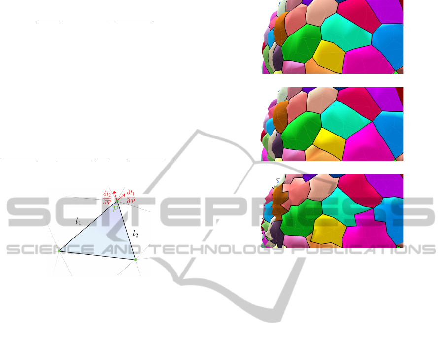
Figure 7: One mesh triangle and the length derivatives used
to compute the local energy gradient at point P.
4.3.2 Energy Balancing
As often in energy-based optimization methods, a lot
of the algorithm’s efficiency relies on the right com-
bination of the weights associated with each energy
term to produce a balanced behavior.
In our case, the energies taken separately have
very different effects, with almost contradictory re-
sults. For instance, considered alone, the image en-
ergy will push the mesh vertices towards the local
maxima of the approximated gradient k∇S k in a con-
verging way : all the vertices in the neighborhood of
one maximum will be attracted by it. This generates
small and possibly irregular triangles as it is visible in
Figure 8 (a), in complete contradiction with the regu-
larity energy.
The same goes for planarity and linearity energies,
as projections on a plane for example might create
flat triangles depending on its original orientation, as
in Figure 8 (b). The regularization energy will then
generally have an antagonist effect on the behavior of
the other forces. It acts as a rigidity constraint trying
to preserve the good properties of the mesh triangles,
through the global displacement induced by the re-
maining energies.
Acting alone however, it fails to produce realistic
cell shapes, leading to noisy edges and irregular cell
(a)
(b)
(c)
Figure 8: Effects of the optimization of the different energy
terms on the mesh : image energy (a) shape prior energy (b)
and regularity energy (c).
facets (as the shape of triangles is optimizes without
regard on the consequences on the surface geometry).
This is clear on the very regular mesh of Figure 8 (c)
where almost equilateral triangles generate very irreg-
ular borders.
It is then very important to balance it well rela-
tively to the shape an image terms to have an evolution
where the influence of the latter is visible (the rigidity
of the mesh should not prevent him from deforming)
while the regularity of the triangles is preserved (and
not crushed by the destructive effects of the other en-
ergies).
To find the weights offering the best compromise
between the intrinsic quality of the mesh and the its
consistency with the data, we used the 7 quality cri-
teria our process is implicitly designed to maximize.
By exploring the value space for the set of parameters
ω, and calculating the correlation of the quality
estimators with the different values, we estimated
a best joint configuration of the energy weights:
• ω
gradient
= 0.17
• ω
plan
= 0.47
• ω
line
= 1.3
• ω
qual
= 2.0
• ω
size
= 0.005
• σ
v
= 1.0
BIOIMAGING2015-InternationalConferenceonBioimaging
30

4.3.3 Optimization Results
We applied our mesh optimization method to tissue
meshes of different shoot apical meristems obtained
form the Delaunay tetrahedral mesh generation. The
cell corners are optimized with their extracted image
position, and the rest of the mesh vertices by energy
gradient descent.
The termination criterion is set to be a fixed num-
ber of iterations rather than a measure of deformation
between two iterations. One of the reasons for this
choice is that the energy minimum for the data attach-
ment energy would be a mesh where vertices concen-
trate at local gradient maxima. Though the regulariza-
tion energy works against this tendency, it is not guar-
anteed to find a globally stable configuration avoiding
this problem, and it was sensible to stop the evolution
as soon as the energies have all had the time to play
their role, with 20 iterations.
Figure 9: Example of the application of our optimization
process on a meristem mesh.
The result of the optimization is a mesh with the
same topology as the initial one, but with a geome-
try that makes it much more consistent with the cell
regions in the image and with their biological reality
at the same time. This better consistency visible in
Figure 9 is achieved without any unnecessary compli-
cation of the mesh, which keeps a constant number of
elements all along the process.
4.4 Implementation Details
The algorithms detailed above were implemented in
Python 2.7, using the standard NumPy and SciPy li-
braries, and wrappers for the C++ CGAL library.
An implementation constraint comes from the fact
that 16-bit labels are not handled by CGAL the mesh
generation function. Consequently, the processing of
images with more that 255 cells requires a re-labeling
step before the mesh generation, and the re-affectation
of original labels to the connected components in the
resulting tetrahedral complex.
Concerning execution times, the complexity
proves to be linear with respect to the number of cells
in the image, as the number of triangles varies pro-
portionally with it. The typical computation times for
a 2000 cell image is of 125s for the mesh generation
and 130s for its optimization, provided the costly fil-
tering of the image necessary for the gradient and the
cell corner extraction (depending on the image size)
has been computed beforehand.
5 EVALUATION
To assess the quality of the reconstructed tissue
meshes, we generated meshes over several segmented
SAM images, and computed the estimators for the
seven quality criteria. We give here a formal defini-
tion of these normalized estimators, using the nota-
tions of our mesh representation:
• Region Consistency (optimized by E
image
) com-
puted using the average volume error, V
M
(c) rep-
resenting the volume of cell c in the mesh and
V
S
(c) in the image:
q
region
= 1 −
1
|W
3
|
∑
c∈W
3
|V
M
(c) −V
S
(c)|
V
S
(c)
• Interest Point Preservation (optimized by E
image
and by cell corner extraction) computed using the
average minimal distance of a cell corner P
0
in the
image to a cell corner of the mesh, normalized by
the maximal 26-neighborhood distance:
q
point
= min
1,
√
3
1
|
Corner
S
|
∑
Corner
S
min
Corner
M
(v)
(kP (v) −P
0
k)
• Cell Convexity (optimized by E
prior
) computed
using the average ratio between the volume V
M
(c)
of the cell c and the volume of the convex hull H
of its vertices:
q
convexity
=
1
|W
3
|
∑
c∈W
3
V
M
(c)
V
H
P (v) | v ∈ B
3
3
(c)
• Surface Arrangement (implicitly optimized)
computed using the average squared deviation of
projected cell angles on the tangent plane at sur-
face cell corners θ
v
(c) to
2π
3
, corresponding to a
regular configuration:
q
angle
= min
1,
√
2 −
1
π/3
v
u
u
t
1
|Corner
M
|
∑
Corner
M
(v)
1
|R
3
0
(v)|
∑
c∈R
3
0
(v)
(θ
v
(c) −
2π
3
)
2
MeshingMeristems-AnIterativeMeshOptimizationMethodforModelingPlantTissueatCellResolution
31
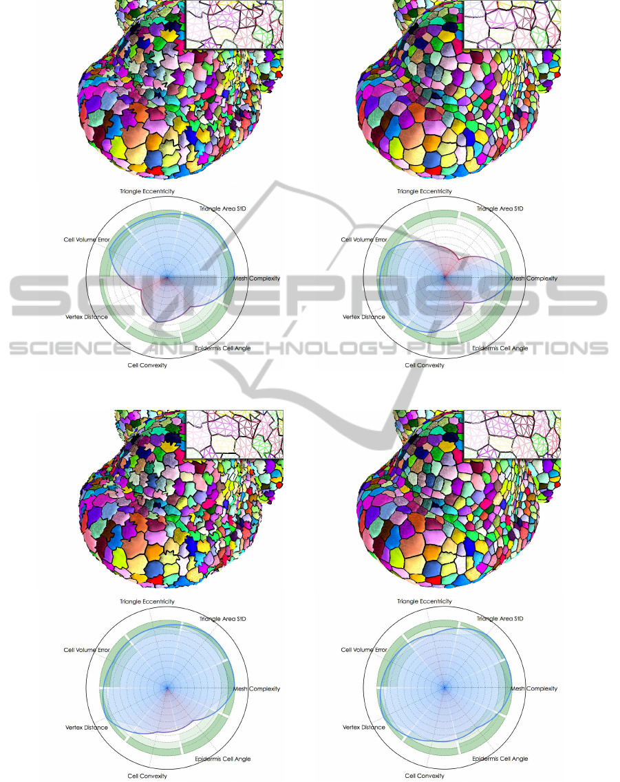
(a) (b)
(c) (d)
Figure 10: Validation of the SAM mesh optimization results through the comparison of average mesh quality estimators on
original meshes (a) and on the corresponding optimized meshes using image attachment energy only (b), using regularity
energy only (c) and with the full energy (d).
BIOIMAGING2015-InternationalConferenceonBioimaging
32

• Triangle Quality (optimized by E
regularity
) com-
puted using the average eccentricity of all the
mesh triangles, estimated using the sum of si-
nuses:
q
triangle
=
1
|W
2
|
∑
t∈W
2
2
3
√
3
∑
v∈B
2
2
(t)
sin
d
P (v)
• Size Homogeneity (optimized by E
regularity
) com-
puted using the standard deviation of the areas A
of all the mesh triangles, normalized by their av-
erage area
¯
A:
q
homogeneity
= min
1,
√
2 −
q
∑
t∈W
2
A(t) −
¯
A
2
∑
t∈W
2
A(t)
• Mesh Lightness (optimized by the distance pa-
rameter of the mesh generation) computed using
the average number of triangle necessary to rep-
resent one cell, normalized by the number n
oct
=
152 obtained for a good triangulation of a space-
filling truncated octahedron:
q
lightness
= min
1,
n
oct
1
card(W
3
)
∑
c∈W
3
card(B
3
(c))
!
(an empirical value of
1
3π
3
q
1
|W
3
|
∑
c∈W
3
V
S
(c) for
the distance parameter proved to give values of
q
lightness
between 0.95 and 1)
Such an evaluation framework opens the way to
a rather exhaustive quantification of the quality of a
SAM tissue mesh, both from an intrinsic point of view
and from the comparison with real-life data. Based
on their typical values on reference quality meshes,
we associated each quality estimator with acceptabil-
ity thresholds, represented as green ranges on the di-
agrams. As such, it constitutes an original tool to as-
sess whether a mesh representing a complex plant cell
tissue satisfies all the necessary computational and vi-
sual properties.
This evaluation framework is also flexible as it can
be adapted to different types of a priori constraints in
the definition of the quality criteria, for instance if one
deals with other types of tissues. In such a case, it is
possible to select and quantify additional criteria for
mesh quality and integrate them in the energy func-
tional as well as on the evaluation spider representa-
tion.
Applied to both the initial meshes and the result-
ing optimized meshes, this evaluation method under-
lines the contribution of our optimization process.
The results, averaged over several images containing
1000 to 3000 cells, are presented in Figure 10. To an-
alyze the results with more precision, we compared
the quality estimators from the initial meshes (Figure
10 (a)), with those achieved by different variants of
the energy:
• Image attachment Energy (Figure 10 (b)): the
minimization of E
image
only leads to a valuable
improvement of cell shapes while providing an
excellent approximation of the image data. How-
ever the geometry of the mesh triangles is de-
stroyed, which is clearly visible in the perfor-
mance over regularity criteria. The apparition
of degenerated triangles penalizes this scores and
gives locally wrong configurations, around cell
corners notably.
• Regularity Energy (Figure 10 (c)): the optimiza-
tion based on the minimization of E
regularity
(along
with the optimal cell corner shifting) appears as
an effective way of preserving, if not improving,
the overall quality of the mesh triangles, through-
out the deformation induced by the motion of the
vertices. Still, the visual impression produced by
this optimization appears very poor, which is con-
firmed by the mitigated performance reached on
the cell shape quality criteria.
• Full Energy (Figure 10 (d)): it appears then
clearly that the addition of the other energy terms
is essential to obtain a globally satisfying result.
The quantitative measures show that regulariza-
tion forces and shape/image forces have antago-
nist effects, the latter tending to improve the cell
shape related criteria with a strong counterpart
on the triangle quality criteria. Their simulta-
neous application constitutes an improvement on
both sides, as the rigidity provided by the regu-
larity term compensates the natural tendency of
the other terms to flatten the triangles, while leav-
ing enough flexibility to allow for both objectively
and visually satisfactory cell reconstructions.
The optimization through the balanced combina-
tion of the different energies appears then as the only
way to obtain an overall optimal compromise that
does not neglect any aspect of the quality criteria. The
result is a mesh that models in a visually convinc-
ing way the shape and disposition of the cells in the
meristem, with a high regularity of the triangles, and a
strong consistency with the original image, while pre-
serving an overall complexity low enough to make it
exploitable for visualization and simulation uses.
6 CONCLUSIONS
The method we presented to reconstruct a complex
triangular mesh of a shoot apical meristem cell tis-
MeshingMeristems-AnIterativeMeshOptimizationMethodforModelingPlantTissueatCellResolution
33

sue actually bridges a gap between experimental data,
and higher-level computational simulations. The
mesh representation we obtain constitutes a ready-to-
process object, including local shape information as
well as tissue-scale topological relations. It opens the
way to a great deal of potential applications, from
fast shape feature extraction using discrete geome-
try, to statistical computations (average shapes, ex-
tended to average tissue) or physical and mechani-
cal growth simulations. Using growing real-world ex-
amples rather than hand-built model structures would
constitute a major step for the validation of such bio-
physical development models.
All of this of course holds only if the provided re-
construction presents the properties needed to make
these applications possible and sensible. Our opti-
mization process guarantees that the produced mesh
reconstructs faithfully the experimental data, with a
complexity that will make processing times reason-
able, and by geometrical elements regular enough to
expect correct simulations. The quantitative quality
evaluation framework we designed ensures that the
compromise between these hardly consonant aspects
fulfills the necessary criteria. It additionally provides
an objective and complete measure of the quality of
a SAM tissue mesh, that could be used to compare
different methods.
A further improvement in mesh quality could
be reached by optimizing simultaneously the mesh
topology along with its geometry, and perform oper-
ations of vertex insertion and suppression based on
the same energy minimization process. Such an ap-
proach would allow to dynamically improve the local
topology (that now may still lead to noisy cell edges)
and optimize the mesh lightness along with the other
quality criteria.
The performance reached by the mesh optimiza-
tion method we described is already enough to con-
sider that the step of converting an image in a higher-
level representation is crossed, and the ensuing ap-
plications in computation and simulation at reach. It
constitutes in any way an additional tool of great in-
terest for the better understanding of plant morpho-
genesis.
REFERENCES
Amenta, N., Bern, M. W., and Eppstein, D. (1997). Optimal
point placement for mesh smoothing. In Proceedings
of the ACM-SIAM Symposium on Discrete Algorithms,
pages 528–537.
Barbier de Reuille, P., Bohn-Courseau, I., Godin, C., and
Traas, J. (2005). A protocol to analyse cellular dy-
namics during plant development. The Plant Journal,
44(6):1045–1053.
Barbier de Reuille, P., Robinson, S., and Smith, R. S.
(2014). Quantifying cell shape and gene expression
in the shoot apical meristem using MorphoGraphX.
In Plant Cell Morphogenesis, pages 121–134.
Chakraborty, A., Perales, M. M., Reddy, G. V., and
Roy Chowdhury, A. K. (2013). Adaptive geomet-
ric tessellation for 3d reconstruction of anisotropically
developing cells in multilayer tissues from sparse vol-
umetric microscopy images. PLoS One, 8(8).
Chakraborty, A., Yadav, R., Reddy, G. V., and Roy Chowd-
hury, A. K. (2011). Cell resolution 3d reconstruction
of developing multilayer tissues from sparsely sam-
pled volumetric microscopy images. In BIBM, pages
378–383.
Chan, T. and Vese, L. (2001). Active contours with-
out edges. IEEE Transactions on Image Processing,
10(2):266–277.
Dufour, A., Thibeaux, R., Labruyere, E., Guillen, N., and
Olivo-Marin, J.-C. (2011). 3-d active meshes: Fast
discrete deformable models for cell tracking in 3-d
time-lapse microscopy. IEEE Transactions on Image
Processing, 20(7).
Fernandez, R., Das, P., Mirabet, V., Moscardi, E., Traas, J.,
Verdeil, J.-L., Malandain, G., and Godin, C. (2010).
Imaging plant growth in 4D : robust tissue reconstruc-
tion and lineaging at cell resolution. Nature Methods,
(7):547–553.
Field, D. A. (1988). Laplacian smoothing and delaunay tri-
angulations. Communications in Applied Numerical
Methods, 4(6):709–712.
Field, D. A. (2000). Qualitative measures for initial meshes.
International Journal for Numerical Methods in Engi-
neering, 47(4):887–906.
Freitag, L. A. (1997). On combining laplacian and
optimization-based mesh smoothing techniques. In
Trends in Unstructured Mesh Generation, pages 37–
43.
Guignard, L., Godin, C., Fiuza, U.-M., Hufnagel, L.,
Lemaire, P., and Malandain, G. (2014). Spatio-
temporal registration of embryo images. In IEEE In-
ternational Symposium on Biomedical Imaging.
Hoppe, H., DeRose, T., Duchamp, T., McDonald, J., and
Stuetzle, W. (1993). Mesh optimization. In Pro-
ceedings of the 20th Annual Conference on Computer
Graphics and Interactive Techniques, SIGGRAPH
’93, pages 19–26.
Kass, M., Witkin, A., and Terzopoulos, D. (1988). Snakes:
Active contour models. International Journal of Com-
puter Vision, 1(4):321–331.
Keller, P. J. (2013). Imaging morphogenesis: Technological
advances and biological insights. Science, 340(6137).
Kwiatkowska, D. (2004). Surface growth at the reproduc-
tive shoot apex of Arabidopsis thaliana pin-formed
1 and wild type. Journal of Experimental Botany,
55(399):1021–1032.
Lorensen, W. E. and Cline, H. E. (1987). Marching cubes:
A high resolution 3d surface construction algorithm.
In Proceedings of the 14th Annual Conference on
BIOIMAGING2015-InternationalConferenceonBioimaging
34

Computer Graphics and Interactive Techniques, SIG-
GRAPH ’87, pages 163–169.
Michelin, G., Guignard, L., Fiuza, U.-M., Malandain, G.,
et al. (2014). Embryo cell membranes reconstruction
by tensor voting. In IEEE International Symposium
on Biomedical Imaging.
Owen, S. J. (1998). A survey of unstructured mesh
generation technology. In International Meshing
Roundtable, pages 239–267.
Rizzi, B. and Peyrieras, N. (2014). Towards 3d in silico
modeling of the sea urchin embryonic development.
Journal of Chemical Biology, 7(1):17–28.
Robin, F. B., Dauga, D., Tassy, O., Sobral, D., Daian, F., and
Lemaire, P. (2011). Time-lapse imaging of live Phal-
lusia embryos for creating 3d digital replicas. Cold
Spring Harbor Protocols, 1244(6).
Shewchuk, J. R. (1998). Tetrahedral mesh generation by
Delaunay refinement. In Proceedings of the Four-
teenth Annual Symposium on Computational Geom-
etry, SCG ’98, pages 86–95.
Tataw, O. M., Reddy, G. V., Keogh, E. J., and Roy Chowd-
hury, A. K. (2013). Quantitative analysis of live-cell
growth at the shoot apex of arabidopsis thaliana: Al-
gorithms for feature measurement and temporal align-
ment. IEEE/ACM Trans. Comput. Biology Bioinform.,
10(5):1150–1161.
CGAL (1996). CGAL, Computational Geometry Algorithms
Library. http://www.cgal.org.
Vidal, V., Wolf, C., and Dupont, F. (2012). Combinatorial
mesh optimization. The Visual Computer, 28(5):511–
525.
MeshingMeristems-AnIterativeMeshOptimizationMethodforModelingPlantTissueatCellResolution
35
