
A Shuffled Complex Evolution Based Algorithm for Examination
Timetabling
Benchmarks and a New Problem Focusing Two Epochs
Nuno Leite
1,3,∗
, Fernando Mel
´
ıcio
3
and Agostinho C. Rosa
2,3
1
Instituto Superior de Engenharia de Lisboa/ADEETC, Polytechnic Institute of Lisbon,
Rua Conselheiro Em
´
ıdio Navarro, n.° 1, 1959-007, Lisboa, Portugal
2
Department of Bioengineering/Instituto Superior T
´
ecnico, Universidade de Lisboa,
Av. Rovisco Pais, n.° 1, 1049-001 Lisboa, Portugal
3
Institute for Systems and Robotics/LaSEEB, Instituto Superior T
´
ecnico, Universidade de Lisboa,
Av. Rovisco Pais, n.° 1, TN 6.21, 1049-001, Lisboa, Portugal
Keywords:
Examination Timetabling, Shuffled Complex Evolution Algorithm, Memetic Computing, Great Deluge
Algorithm, Toronto Benchmarks, Two-Epoch Examination Timetabling.
Abstract:
In this work we present a memetic algorithm for solving examination timetabling problems. Two problems
are analysed and solved. The first one is the well-studied single-epoch problem. The second problem studied
is an extension of the standard problem where two examination epochs are considered, with different dura-
tions. The proposed memetic algorithm inherits the population structure of the Shuffled Complex Evolution
algorithm, where the population is organized into sets called complexes. These complexes are evolved in-
dependently and then shuffled in order to generate the next generation complexes. In order to explore new
solutions, a crossover between two complex’s solutions is done. Then, a random solution selected from the
top best solutions is improved, by applying a local search step where the Great Deluge algorithm is employed.
Experimental evaluation was carried out on the public uncapacitated Toronto benchmarks (single epoch) and
on the ISEL-DEETC department examination benchmark (two epochs). Experimental results show that the
proposed algorithm is efficient and competitive on the Toronto benchmarks with other algorithms from the
literature. Relating the ISEL-DEETC benchmark, the algorithm attains a lower cost when compared with the
manual solution.
1 INTRODUCTION
The Examination Timetabling Problem (ETTP) is a
combinatorial optimisation problem which objective
is to allocate course exams to a set of limited time
slots, while respecting some hard constraints, such
as respect maximum room capacity, guarantee room
exclusiveness for given exams, guarantee that no stu-
dents will sit two or more exams at the same time
slot, guarantee exam ordering (e.g. larger exams
must be scheduled at the beginning of the timetable),
among others (McCollum et al., 2012). The ETTP
is a multi-objective problem in nature as several ob-
jectives (reflecting the various interested parties, e.g.,
students, institution, teachers) are considered (Burke
et al., 2008). However, due to complexity reasons, the
∗
This work was supported by the FCT – Fundac¸
˜
ao para a
Ci
ˆ
encia e a Tecnologia Project PEst-OE/EEI/LA0009/2013 and by
the FCT grant Ref. No. SFRH/PROTEC/67953/2010.
ETTP has been dealt as a single-objective problem. A
second type of constraints, named soft constraints, are
also considered but there is no obligation to observe
them. The optimisation goal is usually the minimisa-
tion of the soft constraints violations.
The ETTP, as other problems (e.g. Course
timetabling) belong to the general class of timetabling
problems which include Transportation and Sports
timetabling, Nurse scheduling, among others. In
terms of complexity, University timetabling problems
belong to the NP-complete class of problems (Qu
et al., 2009). In the past 30 years, several heuris-
tic solution methods have been proposed to solve the
ETTP. The meta-heuristics form the most success-
ful methods applied to ETTP. These are mainly di-
vided into two classes (Talbi, 2009): single-solution
based meta-heuristics and population-based meta-
heuristics. Single-solution meta-heuristics include al-
gorithms such as simulated annealing, tabu search,
112
Leite N., Melício F. and Rosa A..
A Shuffled Complex Evolution Based Algorithm for Examination Timetabling - Benchmarks and a New Problem Focusing Two Epochs.
DOI: 10.5220/0005164801120124
In Proceedings of the International Conference on Evolutionary Computation Theory and Applications (ECTA-2014), pages 112-124
ISBN: 978-989-758-052-9
Copyright
c
2014 SCITEPRESS (Science and Technology Publications, Lda.)

and variable neighbourhood search. Population-
based meta-heuristics include genetic algorithms, ant
colony optimisation, particle swarm optimisation and
memetic algorithms. Particle swarm optimisation
integrates the larger branch named Swarm Intelli-
gence (Kamil et al., 1987). In Swarm Intelligence
the behaviour of self-organised systems (e.g., frog
swarm in a swamp, fish swarm, honeybee mating)
is simulated. For a recent survey of approaches ap-
plied to the ETTP see (Qu et al., 2009). Population-
based approaches, especially hybrid methods that em-
ploy single-solution meta-heuristics in an exploitation
phase, form the most successful methods. These hy-
brid methods are named Memetic Algorithms (Neri
et al., 2012), and integrate the larger branch known
as Memetic Computing. In the literature, several
population-based methods were proposed for solv-
ing the ETTP: ant colony (Dowsland and Thompson,
2005), particle swarm optimisation (Chu et al., 2006),
fish swarm optimisation algorithm (Turabieh and Ab-
dullah, 2011a; Turabieh and Abdullah, 2011b), and
honeybee mating optimisation (Sabar et al., 2009).
In previous research undertaken (Leite et al.,
2013), the ETTP was approached by an adaptation of
the Shuffled Frog-Leaping Algorithm (SFLA) (Eusuff
et al., 2006). The SFLA is, by its turn, based on the
Shuffled Complex Evolution (SCE) approach (Duan
et al., 1993). Both are evolutionary algorithms (EA)
containing structured populations and an efficient ex-
ploitation phase (local search). They were success-
fully applied to Global optimisation problems.
An important feature that must be observed when
designing an EA-based approach is the diversity man-
agement (Neri, 2012), as a poor population diversity
leads the algorithm to stagnate prematurely. Another
emergent approach that uses a structured population
is the Cellular Genetic Algorithm (cGA) (Alba and
Dorronsoro, 2008), which promotes a smooth actual-
ization of solutions through the population, therefore
maintaining the diversity.
In this work, we propose a memetic algorithm for
solving combinatorial optimisation problems. In the
presented work, we show its application to the ETTP.
The method, coined SCEA – Shuffled Complex Evo-
lution Algorithm, inherits features from the SCE and
SFLA approaches, namely the population is orga-
nized into sub-populations called complexes (meme-
plexes in SFLA). Population diversity is maintained
in the SCEA using both a crossover operator and a
special solution update mechanism. The method is
hybridised with the single-solution method Great Del-
uge Algorithm (GDA) (Dueck, 1993). The GDA is
a simulated annealing variant which comprises a de-
terministic acceptance function of neighbouring solu-
Table 1: Hard and Soft constraints for the uncapacitated
ETTP considered in this work. The H
2
constraint appears
in the two-epoch formulation.
Constraint Explanation
and Type
H
1
(Hard) There cannot exist students sitting for
more than one exam simultaneously.
H
2
(Hard) A minimum distance between the two
exams of a course must be observed.
S
1
(Soft) The exams should be spread out
evenly through the timetable.
tions.
There exist several public benchmarks available
for algorithm testing and comparison purposes. The
most used are the Toronto, and the International
Timetabling Competition 2007 (ITC 2007) bench-
marks (Qu et al., 2009). The SCEA is applied to
the uncapacitated Toronto benchmarks (Carter et al.,
1996), comprising 13 ETTP real instances (single ex-
amination epoch), and also to the uncapacitated ETTP
instance of the Electrical, Telecommunications and
Computer Department at the Lisbon Polytechnic In-
stitute (ISEL-DEETC), which comprises two exami-
nation epochs.
The paper is organized as follows. Section 2
presents the ETTP formulations of the considered
ETTP instances. In Section 3 we describe the pro-
posed memetic algorithm for solving the ETTP. Sec-
tion 4 presents simulation results and analysis on the
algorithm performance. Finally, conclusions and fu-
ture work are presented in Section 5.
2 EXAMINATION TIMETABLING
PROBLEMS
In this section we describe in more detail the two
ETTP problems analysed in this work. The first prob-
lem is the well-studied single-epoch problem, where
a single examination epoch with fixed number of time
slots is considered. The second problem is a new
problem emerged from practice, where two examina-
tion epochs are considered, with different number of
time slots allotted for each epoch.
Table 1 describe the hard and soft constraints of
the ETTP instances analysed in this work.
2.1 The Single-epoch Problem
The single-epoch problem standard formulation was
adapted from (Abdullah et al., 2009) and (Burke et al.,
AShuffledComplexEvolutionBasedAlgorithmforExaminationTimetabling-BenchmarksandaNewProblemFocusing
TwoEpochs
113

2004)), and is presented next. The following terms
were defined:
• E
i
, is the set of N examinations (i = 1, ..., N);
• T , is the number of time slots;
• C = (c
i j
)
N×N
(Conflict matrix), is a symmetric
matrix of size N where each element, denoted by
c
i j
(i, j ∈ {1,...,N}), represents the number of
students attending exams i and j;
• M, is the total number of students;
• t
k
(1 ≤ t
k
≤ T ) denotes the assigned time slot for
exam k (k ∈ {1, .. ., N}).
The optimisation objective is the minimisation of the
sum of proximity costs given by:
minimise f
c
=
1
M
·
N−1
∑
i=1
N
∑
j=i+1
c
i j
· prox(i, j) (1)
where
prox(i, j) =
2
5−|t
i
−t
j
|
i f 1 ≤ |t
i
−t
j
| ≤ 5
0 otherwise ,
(2)
subject to
N−1
∑
i=1
N
∑
j=i+1
c
i j
· λ(t
i
,t
j
) = 0 and (3)
λ(t
i
,t
j
) =
1 i f t
i
= t
j
0 otherwise
.
Equation (2) measures the proximity cost of exams i
and j which is greater than zero for exams that are
five or less time slots apart. Equation (3) represents
the hard constraint H
1
. Equation (1) represents the
soft constraint S
1
.
2.1.1 Toronto Datasets
As previously mentioned in Section 1, for the single-
epoch problem, we use in our simulations the Unca-
pacitated Toronto benchmarks, Version I (Table 2).
2.2 The Two-epoch Problem
The two-epoch problem is an extension of the stan-
dard problem where two examination epochs of dif-
ferent dimensions are considered instead of just a
single epoch. A snapshot of timetables having two
epochs is given in Tables 8 and 9.
A new hard constraint (constraint H
2
in Table 1)
is specified in the two-epoch problem for guarantee-
ing a minimum number of time slots between the two
examinations of the same course, in order to give the
necessary study time, exam correction and proofing.
In the two-epoch problem formulation, the following
terms were added to the single-epoch problem formu-
lation:
Table 2: Specifications of the uncapacitated Toronto bench-
marks (version I).
Data Students Exams Conflict Time slots
set density
car91 16925 682 0.13 35
car92 18419 543 0.14 32
ear83 1125 190 0.27 24
hec92 2823 81 0.42 18
kfu93 5349 461 0.06 20
lse91 2726 381 0.06 18
pur93 30032 2419 0.03 42
rye92 11483 486 0.07 23
sta83 611 139 0.14 13
tre92 4360 261 0.18 23
uta92 21266 622 0.13 35
ute92 2749 184 0.08 10
yor83 941 181 0.29 21
• T and L, are, respectively, the number of time
slots of the first epoch and the total number of
time slots (sum of the first and second epochs’s
time slots). The number of time slots of the sec-
ond epoch is then L − T ;
• C
relax
= (c
relax
i j
)
N×N
(Relaxed conflict matrix), is
a relaxed version of the conflict matrix C. This
matrix is used in the generation of the second ex-
amination epoch. Further details are given below.
• u
k
(T +1 ≤ u
k
≤ L) denotes the assigned time slot
for exam k (k ∈ {1,..., N}) in the second exami-
nation epoch.
The hard constraint H
2
is specified by:
u
k
−t
k
≥ L
min
, (4)
where L
min
is the minimum time slot distance between
the first and second epoch exams of a given course.
The devised algorithm for solving the two-epoch
problem executes the following steps:
1. Treat the two epochs as two distinct single-epoch
problems. Solve the second epoch problem by
considering the standard single-epoch formula-
tion presented in Section 2.1, but using the relaxed
conflict matrix, C
relax
;
2. Then, solve the first epoch problem using the stan-
dard formulation as depicted in Section 2.1 with
the added constraint H
2
, that is, by adding Eq. (4).
3. At the end of the optimisation step, we join the
two timetables forming the two-epoch timetable
that respects both H
1
and H
2
constraints. The
cost of the two-epoch timetables is the sum of the
costs of the individual timetables.
ECTA2014-InternationalConferenceonEvolutionaryComputationTheoryandApplications
114

Table 3: Characteristics of the DEETC dataset.
Parameter Value
Number of exams 80
Number of students 1238
Number of enrolments 4548
Conflict matrix density
1st epoch 0.32
2nd epoch 0.31
Number of time slots
1st epoch 18
2nd epoch 12
Some final details are now given. In the ISEL-
DEETC dataset, the second epoch is more constrained
than the first epoch, having less time slots (18 and
12 time slots, respectively, for the first and second
epochs). In order to be possible to generate feasible
initial solutions for the second epoch, some entries
(with very few students enrolled) were set to zero,
resulting in a relaxed conflict matrix. However, this
pre-processing is problem dependent and for that rea-
son not obligatory. The algorithm starts by generating
the second examination epoch followed by the gener-
ation of the first examination epoch (with the added
constraint H
2
), but this order is not strict. We could
have started by the inverse order. However, this latter
experiment was not carried out in this work.
In order to optimise the first epoch while respect-
ing the hard constraint H
2
, we have to apply modified
versions of the initialisation procedure, the crossover
and the neighbourhood operators. These modified
versions work with feasible timetables that satisfy
both hard constraints, H
1
and H
2
. As a final detail, we
mention that while we optimised the timetables using
the proximity cost specified in Eq. (2), which mea-
sures conflicts in a neighbourhood of five time slots,
in our collected results we use the measure published
in (Leite et al., 2012), which only considers conflicts
from two consecutive time slots, and do not consider
conflicts on Saturdays. We use this later measure here
in order to be able to compare results with the method
published in (Leite et al., 2012).
2.2.1 ISEL-DEETC Dataset
The problem instance considered in this work is
the DEETC timetable of the winter semester of the
2009/2010 academic year. This benchmark data is de-
tailed in (Leite et al., 2012). The DEETC timetable
comprises five programs: three B.Sc. programs
(named LEETC, LEIC and LERCM) and two M.Sc.
programs (named MEIC and MEET). B.Sc. and
M.Sc. programs have six and four semesters dura-
tion, respectively. The DEETC dataset characteristics
are listed in Table 3.
3 SHUFFLED COMPLEX
EVOLUTION ALGORITHM
FOR EXAMINATION
TIMETABLING
In this section we describe the SCEA algorithm for
solving the ETTP. The SCEA is based on ideas from
the SCE (Duan et al., 1993) and the SFLA (Eusuff
et al., 2006) approaches. In the SCE, the population
is organized into complexes whereas in the SFLA it is
organized into memeplexes. In the text, we use these
two terms interchangeably.
In the SCE and SFLA approaches, global search is
managed as a process of natural evolution. The sam-
ple points form a population that is partitioned into
distinct groups called complexes (memeplexes). Each
of these evolve independently, by searching the space
into different directions. After completing a certain
number of generations, the complexes are combined,
and new complexes are formed through the process of
shuffling. These procedures enhance survivability by
a sharing of information about the search space, con-
structed independently by each complex (Duan et al.,
1993).
The SCEA main steps are illustrated in Figure 1,
whereas the SCEA local search step is depicted in
Figure 2. The main loop of SCEA is identical to
the SCE and SFLA main loop, where complexes are
formed by creating random initial solutions that span
the search space. Here, instead of points, the solutions
correspond to complete and feasible timetables.
The local search step (Figure 2) was fully re-
designed from the SCE and SFLA methods, in or-
der to operate with ETTP solutions. Like SFLA, we
maintain the best and worst solutions of the meme-
plex, denoted respectively as P
b
and P
w
, and elitism is
achieved by maintaining the best global solution, de-
noted as P
g
. The local search step starts by selecting,
randomly, and according with crossover probability
cp, two parent solutions, P
1
and P
2
, for recombina-
tion in order to produce a new offspring. P
1
must
be different from the complex’s best solution. The
solution P
1
is recombined with solution P
2
(see the
crossover operation depicted in Figure 3) and the re-
sulting offspring replaces the parent P
1
. After this,
the complex is sorted in order of increasing objective
function value. The crossover operator was adapted
from the crossover operator of (Abdullah et al., 2010;
Sabar et al., 2009).
After the crossover, a solution in the complex is
selected for improvement according to an improve
probability, ip. The solution is improved by employ-
ing the local search meta-heuristic GDA (Great Del-
AShuffledComplexEvolutionBasedAlgorithmforExaminationTimetabling-BenchmarksandaNewProblemFocusing
TwoEpochs
115
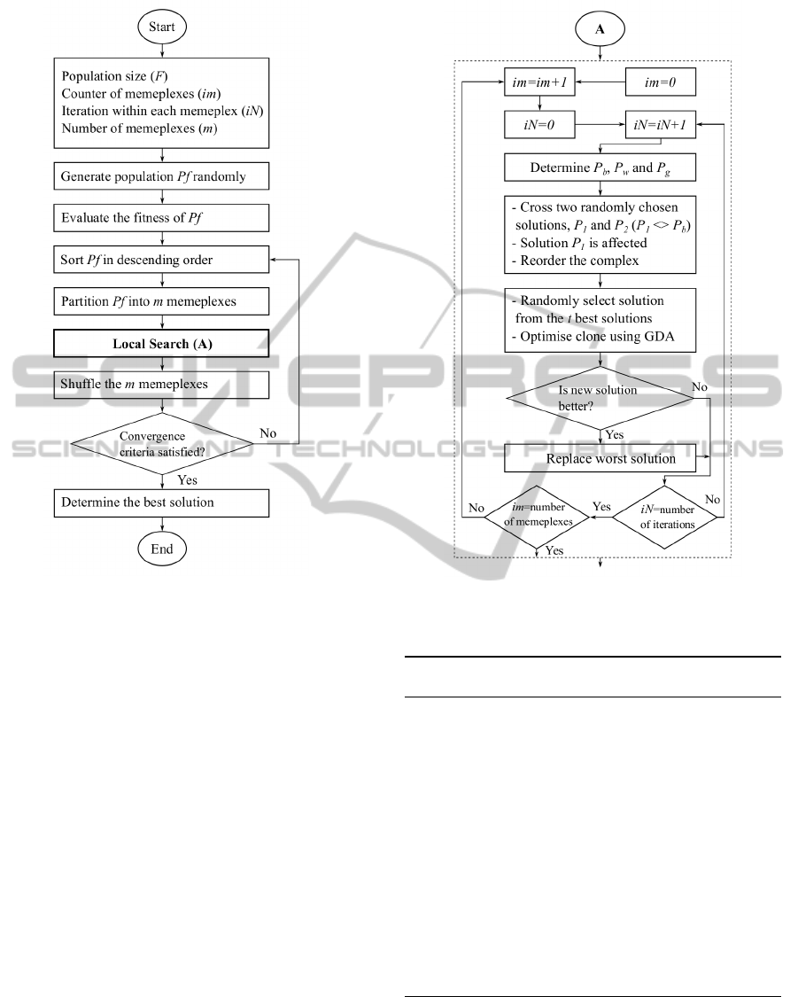
Figure 1: SCEA main steps.
uge Algorithm) (Dueck, 1993). The template of GDA
is presented in Algorithm 3.1. The GDA mimics the
exploration made by a climber trying to reach the top
of a mountain while is raining incessantly. This sce-
nario leads to the name of the algorithm: great deluge.
As the rain never stops, the water level gradually in-
creases until it reaches the climber. The goal of the
climber is finding the way to the top (maximisation
problem) before is reached by the water level. It can
go up or down from that is always above the water
level.
The selection of the solution to improve is made
on the group of the top t best solutions. The exploita-
tion using GDA is done on a clone of the original so-
lution, selected from this group. If the optimised so-
lution is better than the original, then it will replace
the complex’s worst solution. This updating step in
conjunction with the crossover operator guarantees a
reasonable diversity, in an implicit fashion.
The GDA was integrated in the SCEA in the fol-
lowing fashion. We use as the initial solution s
0
the
chosen solution to improve. The level LEV EL is set to
the fitness value of this initial solution s
0
. The search
stops when the water level is equal to the solution fit-
Figure 2: SCEA Local search step.
ness.
Algorithm 3.1: Template of the Great Deluge Algo-
rithm.
Input:
• s
0
/∗ Initial solution ∗/
• Initial water level LEVEL
• Rain speed UP / ∗ U P > 0 ∗ /
1: s = s
0
; /∗ Generation of the initial solution ∗/
2: repeat
3: Generate a random neighbour s
0
;
4: If f (s
0
) < LEV EL Then s = s
0
/∗ Accept
5: the neighbour solution ∗/
6: LEVEL = LEV EL −UP; /∗ update the water
7: level ∗/
8: until Stopping criteria satisfied
9: Output: Best solution found.
Initial Solution Construction
The construction of the initial feasible solutions is
done by a heuristic algorithm which uses the Satu-
ration Degree graph colouring heuristic (Carter et al.,
ECTA2014-InternationalConferenceonEvolutionaryComputationTheoryandApplications
116

t
1
e
2
e
14
e
10
e
3
e
16
t
2
e
1
e
11
e
4
t
3
e
9
e
20
e
5
e
18
t
4
e
6
e
13
e
7
t
5
e
8
e
12
e
15
e
17
e
19
(a) Solution P
1
t
1
e
15
e
20
t
2
e
9
e
2
e
12
e
10
e
7
t
3
e
6
e
1
e
17
e
13
t
4
e
5
e
18
e
4
e
16
t
5
e
8
e
14
e
11
e
3
e
19
(b) Solution P
2
t
1
e
2
e
14
e
10
e
3
e
16
t
2
e
1
e
11
e
4
e
8
e
14
e
11
e
3
e
19
t
3
e
9
e
20
e
5
e
18
t
4
e
6
e
13
e
7
t
5
e
8
e
12
e
15
e
17
e
19
(c) New solution P
1
Figure 3: Crossover between P
1
and P
2
. The resulting solu-
tion P
1
in (c) is the result of combining the solution P
1
(a)
with other solution P
2
(b). The operator inserts into P
1
, at a
random time slot (shown dark shaded in (a) and (c)), exams
chosen from a random time slot from solution P
2
(shown
dark shaded in (b)). When inserting these exams (shown
light gray in (c)), some could be infeasible or already exist-
ing in that time slot (respectively, the case of e
8
and e
11
in
(c)). These exams are not inserted. The duplicated exams
in the other time slots are removed.
1996).
GDA’s Neighbourhood
In the local search with GDA we used the Kempe
chain neighbourhood (Demeester et al., 2012).
Two-epoch Feasibility
In order to be able to execute the SCEA on the two-
epoch problem, we have to implement a different ver-
sion of the initialisation procedure, and the crossover
and neighbourhood operators, that could manage the
hard constraint H
2
mentioned in Section 2. This dif-
ferent version is executed in the first epoch genera-
tion, while the original version is executed in the sec-
ond epoch generation.
4 EXPERIMENTS AND
COMPARISONS
4.1 Problem Instances and
Experimental Settings
The performance of the SCEA was evaluated
using the Toronto datasets (see Table 2). All
these 13 instances can be downloaded from
ftp://ftp.mie.utoronto.ca/pub/carter/testprob. We
also solved the two-epoch ISEL-DEETC instance
(Table 3). For the ISEL-DEETC, there’s a manual
solution available (for the five timetables corre-
sponding to the five engineering programs) from
the ISEL academic services. The algorithm is
programmed in the C++ language. The implemented
code uses the ParadisEO framework (Talbi, 2009).
The hardware and software specifications are: Intel
Core i7-2630QM, CPU @ 2.00 GHz × 8, with 8 GB
RAM; OS: Ubuntu 14.04, 64 bit; Compiler used:
GCC v. 4.8.2.
The parameters of SCEA are: Population size
F = 24, Memeplex count m = 3, Memeplex size n = 8
(no sub-memeplexes were defined), and Number of
time loops (convergence criterion) L = 100000000.
The number of best solutions to consider for selec-
tion on a complex is given by t = n/4 = 2. The
Great Deluge parameter, UP, was set to: UP = 1e−7.
The crossover and improvement probabilities, respec-
tively, cp and ip, were set equal to 0.2 and 1.0. The
parameter values were chosen empirically. To obtain
our simulation results, the SCEA was run five times
on each instance with different random seeds. The
running time of the algorithm was limited to 24 hours
to all datasets except for the pur93. For this larger
dataset, the running time was limited to 48 hours.
4.2 Comparative Results and Discussion
Tables 4 and 5 show the best results of the SCEA on
the Toronto datasets as well as a selection of the best
results available in the literature. The listed meth-
ods include only results validated by (Qu et al., 2009)
(dated until 2008). In the last two rows of each ta-
ble, the TP and TP (11) indicate, respectively, the total
penalty for the 13 instances and the total penalty ex-
cept the pur93 and rye92 instances. Tables 6 and 7
compare SCEA with the top six best algorithms. For
the SCEA we present the lowest penalty value f
min
,
the average penalty value f
ave
, and the standard devi-
ation σ over five independent runs. For the reference
algorithms we present the best and average (where
available) results and the number of runs. Figure 4
illustrate the SCEA evolution on the yor83 dataset.
The authors analysed in Tables 6 and 7 mention
computation times that are within several minutes – 1
hour, to several hours (12 hours maximum).
The best results obtained by SCEA are competi-
tive with the ones produced by state-of-the-art algo-
rithms. It attains a new lower bound on the yor83
dataset. We also observe that the SCEA obtains the
lowest sum of average cost on the TP and TP (11)
AShuffledComplexEvolutionBasedAlgorithmforExaminationTimetabling-BenchmarksandaNewProblemFocusing
TwoEpochs
117

Table 4: Simulation results of SCEA and comparison with selection of best algorithms from literature. Values in bold represent
the best results reported. “–” indicates that the corresponding instance is not tested or a feasible solution cannot be obtained.
Dataset (Carter et al.,
1996)
(Burke and
Newall,
2002)
(Merlot
et al., 2003)
(Burke and
Newall,
2004)
(Burke et al.,
2004)
(Kendall
and Hussin,
2005)
car91 7.10 4.65 5.10 5.00 4.80 5.37
car92 6.20 4.10 4.30 4.30 4.20 4.67
ear83 36.40 37.05 35.10 36.20 35.40 40.18
hec92 10.80 11.54 10.60 11.60 10.80 11.86
kfu93 14.00 13.90 13.50 15.00 13.70 15.84
lse91 10.50 10.82 10.50 11.00 10.40 –
pur93 3.90 – – – 4.80 –
rye92 7.30 – 8.40 – 8.90 –
sta83 161.50 168.73 157.30 161.90 159.10 157.38
tre92 9.60 8.35 8.40 8.40 8.30 8.39
uta92 3.50 3.20 3.50 3.40 3.40 –
ute92 25.80 25.83 25.10 27.40 25.70 27.60
yor83 41.70 37.28 37.40 40.80 36.70 –
TP (11) 327.10 325.45 310.80 325.00 312.50 –
TP 338.30 – – – 326.20 –
Dataset (Yang and
Petrovic,
2005)
(Burke and
Bykov,
2006)
(Eley, 2006) (Burke and
Bykov,
2008)
(Abdullah
et al., 2009)
(Sabar et al.,
2009)
car91 4.50 4.42 5.20 4.58 4.42 4.79
car92 3.93 3.74 4.30 3.81 3.76 3.90
ear83 33.71 32.76 36.80 32.65 32.12 34.69
hec92 10.83 10.15 11.10 10.06 9.73 10.66
kfu93 13.82 12.96 14.50 12.81 12.62 13.00
lse91 10.35 9.83 11.30 9.86 10.03 10.00
pur93 – – – 4.53 – –
rye92 8.53 – 9.80 7.93 – 10.97
sta83 158.35 157.03 157.30 157.03 156.94 157.04
tre92 7.92 7.75 8.60 7.72 7.86 7.87
uta92 3.14 3.06 3.50 3.16 2.99 3.10
ute92 25.39 24.82 26.40 24.79 24.90 25.94
yor83 36.35 34.84 39.40 34.78 34.95 36.18
TP (11) 308.29 301.36 318.40 301.25 300.32 307.17
TP – – – 313.71 – –
quantities, and the lowest sum of best costs on the TP
quantity, for the Toronto datasets. This demonstrates
that SCEA can optimise very different datasets with
good efficiency. A negative aspect of SCEA is the
time taken compared with other algorithms. The time
taken is a reflex of the high diversity of the method
mixed with the low decreasing rate U P. A low U P
value is needed in order for the GDA to find the best
exam movements. If the UP value is higher, the opti-
misation is faster but with worse results, because the
initial, larger conflict, exams are scheduled into sub
optimal time slots, and thus the remainder exams, as
the water level decreases, could not be scheduled in
the optimal fashion.
4.3 Two-epoch Problem
For the two-epoch problem, we run the SCEA with
the same parameters. The L
min
parameter was set
to L
min
= 10 (first and second epoch examinations
of a given course are 10 time slots apart). Tables 8
and 9 illustrate, respectively, the manual and auto-
ECTA2014-InternationalConferenceonEvolutionaryComputationTheoryandApplications
118

Table 5: Simulation results of SCEA and comparison with selection of best algorithms from literature (continued).
Dataset (Burke
et al.,
2010)
(Abdullah
et al., 2010)
(Turabieh
and Abdul-
lah, 2011a)
(Demeester
et al., 2012)
(Abdullah
and Alzaqe-
bah, 2013)
(Alzaqebah
and Abdul-
lah, 2014)
SCEA
car91 4.90 4.35 4.81 4.52 4.76 4.62 4.41
car92 4.10 3.82 4.11 3.78 3.94 4.00 3.75
ear83 33.20 33.76 36.10 32.49 33.61 33.14 32.62
hec92 10.30 10.29 10.95 10.03 10.56 10.43 10.03
kfu93 13.20 12.86 13.21 12.90 13.44 13.59 12.88
lse91 10.40 10.23 10.20 10.04 10.87 10.75 9.85
pur93 – – – 5.67 – – 4.10
rye92 – – – 8.05 8.81 9.17 7.98
sta83 156.90 156.90 159.74 157.03 157.09 157.06 157.03
tre92 8.30 8.21 8.00 7.69 7.94 8.00 7.75
uta92 3.30 3.22 3.32 3.13 3.27 3.27 3.08
ute92 24.90 25.41 26.17 24.77 25.36 25.16 24.78
yor83 36.30 36.35 36.23 34.64 35.74 35.58 34.44
TP (11) 305.80 305.40 312.84 301.02 306.58 305.60 300.62
TP – – – 314.74 – – 312.70
Table 6: Simulation results of SCEA and comparison with the best algorithms from literature. Values in bold represent the
best results reported. “–” indicates that the corresponding instance is not tested or a feasible solution cannot be obtained.
Dataset (Carter et al.,
1996)
(Burke and
Bykov, 2006)
(Abdullah
et al., 2009)
(five runs)
(Burke et al.,
2010)
f
min
f
min
f
min
f
ave
f
min
car91 7.10 4.42 4.42 4.81 4.90
car92 6.20 3.74 3.76 3.95 4.10
ear83 36.40 32.76 32.12 33.69 33.20
hec92 10.80 10.15 9.73 10.10 10.30
kfu93 14.00 12.96 12.62 12.97 13.20
lse91 10.50 9.83 10.03 10.34 10.40
pur93 3.90 – – – –
rye92 7.30 – – – –
sta83 161.50 157.03 156.94 157.30 156.90
tre92 9.60 7.75 7.86 8.20 8.30
uta92 3.50 3.06 2.99 3.32 3.30
ute92 25.80 24.82 24.90 25.41 24.90
yor83 41.70 34.84 34.95 36.27 36.30
TP (11) 327.10 301.36 300.32 306.36 305.80
TP 338.30 – – – –
matic solutions for the most difficult timetable, the
LEETC timetable. Table 10 shows the comparison
of the manual solution timetables conflicts with two
runs of SCEA. The SCEA could generate timetables
with lower cost comparing with the manual solution.
We note that SCEA optimise the merged timetable
comprising the five timetables and not the individual
timetables, so in some cases, some programs timeta-
bles have worse cost (e.g. Run1, 2nd epoch). The re-
sults produced in the first epoch, are comparable with
the results published in (Leite et al., 2012).
AShuffledComplexEvolutionBasedAlgorithmforExaminationTimetabling-BenchmarksandaNewProblemFocusing
TwoEpochs
119
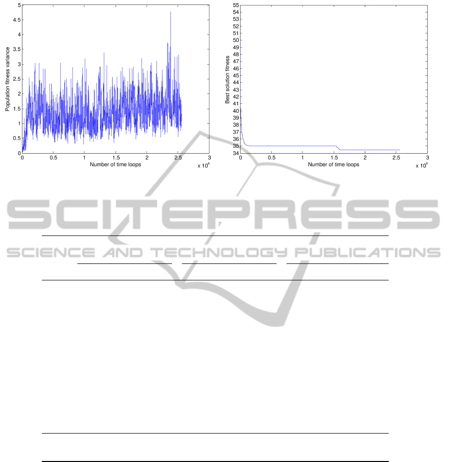
(a) (b)
Figure 4: SCEA evolution on yor83 dataset (a) Population fitness variance evolution along time; (b) Best solution fitness
evolution along time.
Table 7: Simulation results of SCEA and comparison with the best algorithms from literature (continued).
Dataset (Abdullah et al.,
2010) (five runs)
(Demeester et al.,
2012)(20 runs)
SCEA(five runs)
f
min
f
min
f
ave
f
min
f
ave
σ
car91 4.35 4.52 4.64 4.41 4.45 0.03
car92 3.82 3.78 3.86 3.75 3.77 0.01
ear83 33.76 32.49 32.69 32.62 32.69 0.07
hec92 10.29 10.03 10.06 10.03 10.06 0.03
kfu93 12.86 12.90 13.24 12.88 13.00 0.13
lse91 10.23 10.04 10.21 9.85 9.93 0.12
pur93 – 5.67 5.75 4.10 4.17 0.05
rye92 – 8.05 8.20 7.98 8.06 0.06
sta83 156.90 157.03 157.05 157.03 157.03 0.00
tre92 8.21 7.69 7.79 7.75 7.80 0.05
uta92 3.22 3.13 3.17 3.08 3.15 0.05
ute92 25.41 24.77 24.88 24.78 24.81 0.02
yor83 36.35 34.64 34.83 34.44 34.73 0.17
TP (11) 305.40 301.02 302.42 300.62 301.42
TP – 314.74 316.37 312.70 313.65
5 CONCLUSIONS
We presented a memetic algorithm that combines
features from the SCE and the GDA meta-heuristics.
The experimental evaluation of the SCEA shows that
it is competitive with state-of-the-art methods. In
the set of the 13 instances of the Toronto benchmark
data it attains the lowest cost on one dataset, and
the lowest sum of best and average cost with a low
standard deviation. The algorithm main disadvantage
is the time taken on the larger instances.
Further studies should address the diversity man-
agement in order to accelerate the algorithm while
maintaining a satisfactory diversity.
As future research, we intend to apply our solution
method to the instances of the 1st Track (Examination
Timetabling) of the 2nd International Timetabling
Competition (ITC2007), which contain more hard
and soft constraints.
ECTA2014-InternationalConferenceonEvolutionaryComputationTheoryandApplications
120
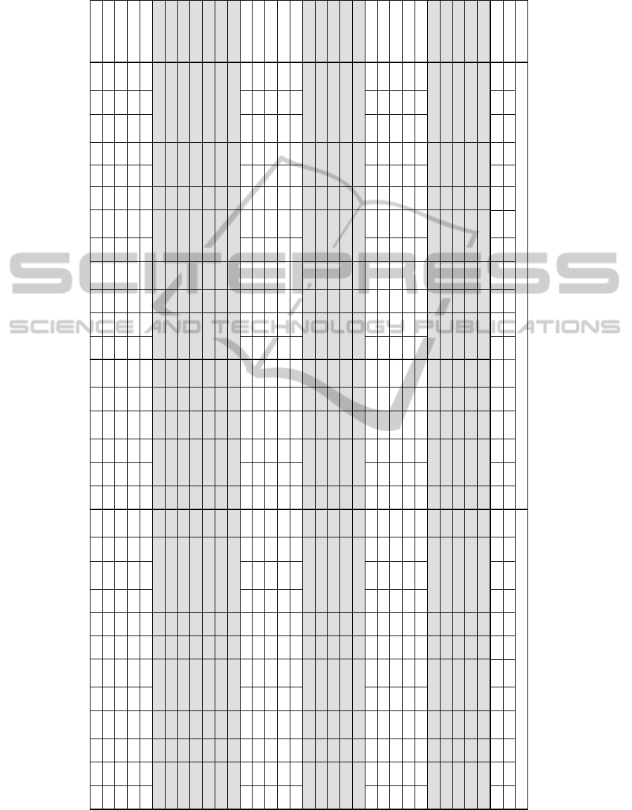
Table 8: Manual solution for the LEETC examination timetable. The courses marked in bold face are shared with other
programs. The number of clashes of this timetable is 287 and 647, respectively, for the first and second epochs.
Course First epoch Second epoch
1 2 3 4 5 6 7 8 9 10 11 12 13 14 15 16 17 18 19 20 21 22 23 24 25 26 27 28 29 30
Mo Tu Wd Tr Fr Sa Mo Tu Wd Tr Fr Sa Mo Tu Wd Tr Fr Sa Mo Tu Wd Tr Fr Sa Mo Tu Wd Tr Fr Sa
ALGA x x
Pg x x
AM1 x x
FAE x x
ACir x x
POO x x
AM2 x x
LSD x x
E1 x x
MAT x x
PE x x
ACp x x
EA x x
E2 x x
SS x x
RCp x x
PICC/CPg x x
PR x x
FT x x
SEAD1 x x
ST x x
RCom x x
RI x x
SE1 x x
AVE x x
SCDig x x
SOt x x
PI x x
SCDist x x
EGP x x
OGE x x
SG x x
AShuffledComplexEvolutionBasedAlgorithmforExaminationTimetabling-BenchmarksandaNewProblemFocusing
TwoEpochs
121
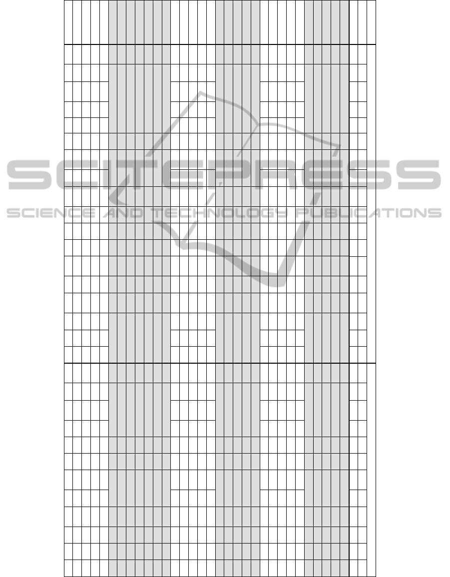
Table 9: Automatic solution for the LEETC examination timetable. The courses marked in bold face are shared with other
programs. The number of clashes of this timetable is 218 and 632, respectively, for the first and second epochs. As can be
observed, all first epoch examinations respect the minimum distance (L
min
= 10) to the corresponding exam time slot in the
second epoch.
Course First epoch Second epoch
1 2 3 4 5 6 7 8 9 10 11 12 13 14 15 16 17 18 19 20 21 22 23 24 25 26 27 28 29 30
Mo Tu Wd Tr Fr Sa Mo Tu Wd Tr Fr Sa Mo Tu Wd Tr Fr Sa Mo Tu Wd Tr Fr Sa Mo Tu Wd Tr Fr Sa
ALGA x x
Pg x x
AM1 x x
FAE x x
ACir x x
POO x x
AM2 x x
LSD x x
E1 x x
MAT x x
PE x x
ACp x x
EA x x
E2 x x
SS x x
RCp x x
PICC/CPg x x
PR x x
FT x x
SEAD1 x x
ST x x
RCom x x
RI x x
SE1 x x
AVE x x
SCDig x x
SOt x x
PI x x
SCDist x x
EGP x x
OGE x x
SG x x
ECTA2014-InternationalConferenceonEvolutionaryComputationTheoryandApplications
122

Table 10: DEETC’s program number of clashes for the manual and automatic two-epoch solutions.
Timetable Manual sol. Automatic sol.
Run 1 Run 2
1st ep. 2nd ep. 1st ep. 2nd ep. 1st ep. 2nd ep.
LEETC 287 647 218 632 261 550
LEIC 197 442 153 480 227 418
LERCM 114 208 83 249 123 195
MEIC 33 63 18 86 15 66
MEET 50 144 20 165 36 124
Combined 549 1163 399 1129 511 1060
Sum 1712 1528 1571
REFERENCES
Abdullah, S. and Alzaqebah, M. (2013). A hybrid self-
adaptive bees algorithm for examination timetabling
problems. Appl. Soft Comput., 13(8):3608–3620.
Abdullah, S., Turabieh, H., and McCollum, B. (2009). A
hybridization of electromagnetic-like mechanism and
great deluge for examination timetabling problems. In
Blesa, M. J., Blum, C., Gaspero, L. D., Roli, A., Sam-
pels, M., and Schaerf, A., editors, Hybrid Metaheuris-
tics, volume 5818 of Lecture Notes in Computer Sci-
ence, pages 60–72. Springer.
Abdullah, S., Turabieh, H., McCollum, B., and McMullan,
P. (2010). A tabu-based memetic approach for exami-
nation timetabling problems. In Yu, J., Greco, S., Lin-
gras, P., Wang, G., and Skowron, A., editors, RSKT,
volume 6401 of Lecture Notes in Computer Science,
pages 574–581. Springer.
Alba, E. and Dorronsoro, B. (2008). Cellular Genetic Algo-
rithms. Springer Publishing Company, Incorporated,
1st edition.
Alzaqebah, M. and Abdullah, S. (2014). An adaptive arti-
ficial bee colony and late-acceptance hill-climbing al-
gorithm for examination timetabling. J. Scheduling,
17(3):249–262.
Burke, E., Bykov, Y., Newall, J., and Petrovic, S. (2004).
A time-predefined local search approach to exam
timetabling problems. IIE Transactions, 36(6):509–
528.
Burke, E., Eckersley, A., McCollum, B., Petrovic, S., and
Qu, R. (2010). Hybrid variable neighbourhood ap-
proaches to university exam timetabling. European
Journal of Operational Research, 206(1):46 – 53.
Burke, E. and Newall, J. (2004). Solving examination
timetabling problems through adaption of heuristic
orderings. Annals of Operations Research, 129(1-
4):107–134.
Burke, E. K. and Bykov, Y. (2006). Solving Exam
Timetabling Problems with the Flex-Deluge Algo-
rithm. In Proceedings of the Sixth International Con-
ference on the Practice and Theory of Automated
Timetabling, pages 370–372. ISBN: 80-210-3726-1.
Burke, E. K. and Bykov, Y. (2008). A late acceptance strat-
egy in Hill-Climbing for exam timetabling problems.
In PATAT ’08 Proceedings of the 7th International
Conference on the Practice and Theory of Automated
Timetabling.
Burke, E. K., McCollum, B., McMullan, P., and Parkes,
A. J. (2008). Multi-objective aspects of the exami-
nation timetabling competition track. Proceedings of
PATAT 2008.
Burke, E. K. and Newall, J. P. (2002). Enhancing timetable
solutions with local search methods. In Burke, E. K.
and Causmaecker, P. D., editors, PATAT, volume 2740
of Lecture Notes in Computer Science, pages 195–
206. Springer.
Carter, M., Laporte, G., and Lee, S. Y. (1996). Examina-
tion Timetabling: Algorithmic Strategies and Appli-
cations. Journal of the Operational Research Society,
47(3):373–383.
Chu, S.-C., Chen, Y.-T., and Ho, J.-H. (2006). Timetable
scheduling using particle swarm optimization. In Pro-
ceedings of the First International Conference on In-
novative Computing, Information and Control - Vol-
ume 3, ICICIC ’06, pages 324–327, Washington, DC,
USA. IEEE Computer Society.
Demeester, P., Bilgin, B., Causmaecker, P. D., and Berghe,
G. V. (2012). A hyperheuristic approach to exami-
nation timetabling problems: benchmarks and a new
problem from practice. J. Scheduling, 15(1):83–103.
Dowsland, A. and Thompson, M. (2005). Ant colony
optimization for the examination scheduling prob-
lem. Journal of the Operational Research Society,
56(4):426–438.
Duan, Q., Gupta, V., and Sorooshian, S. (1993). Shuffled
complex evolution approach for effective and efficient
global minimization. Journal of Optimization Theory
and Applications, 76(3):501–521.
Dueck, G. (1993). New optimization heuristics: The
great deluge algorithm and the record-to-record travel.
Journal of Computational Physics, 104(1):86 – 92.
AShuffledComplexEvolutionBasedAlgorithmforExaminationTimetabling-BenchmarksandaNewProblemFocusing
TwoEpochs
123

Eley, M. (2006). Ant algorithms for the exam timetabling
problem. In PATAT VI, volume 3867 of Lecture Notes
in Computer Science, pages 364–382. Springer.
Eusuff, M., Lansey, K., and Pasha, F. (2006). Shuf-
fled frog-leaping algorithm: a memetic meta-heuristic
for discrete optimization. Engineering Optimization,
38(2):129–154.
Kamil, A., Krebs, J., and Pulliam, H. (1987). Foraging be-
havior. Plenum Press.
Kendall, G. and Hussin, N. (2005). An investigation of
a tabu-search-based hyper-heuristic for examination
timetabling. In Multidisciplinary Scheduling: Theory
and Applications, pages 309–328. Springer US.
Leite, N., Mel
´
ıcio, F., and Rosa, A. (2013). Solving the ex-
amination timetabling problem with the shuffled frog-
leaping algorithm. In Proceedings of the 5th Inter-
national Joint Conference on Computational Intelli-
gence, pages 175–180.
Leite, N., Neves, R. F., Horta, N., Melicio, F., and
Rosa, A. C. (2012). Solving an Uncapacitated Exam
Timetabling Problem Instance using a Hybrid NSGA-
II. In Proceedings of the 4th International Joint Con-
ference on Computational Intelligence, pages 106–
115.
McCollum, B., McMullan, P., Parkes, A. J., Burke, E. K.,
and Qu, R. (2012). A New Model for Automated
Examination Timetabling. Annals of Operations Re-
search, 194:291–315.
Merlot, L., Boland, N., Hughes, B., and Stuckey, P. (2003).
A hybrid algorithm for the examination timetabling
problem. In PATAT IV, volume 2740 of Lecture Notes
in Computer Science, pages 207–231. Springer.
Neri, F. (2012). Diversity management in memetic algo-
rithms. In (Neri et al., 2012), pages 153–165.
Neri, F., Cotta, C., and Moscato, P., editors (2012). Hand-
book of Memetic Algorithms, volume 379 of Studies
in Computational Intelligence. Springer.
Qu, R., Burke, E., McCollum, B., Merlot, L. T. G., and
Lee, S. Y. (2009). A Survey of Search Methodologies
and Automated System Development for Examination
Timetabling. Journal of Scheduling, 12:55–89.
Sabar, N. R., Ayob, M., and Kendall, G. (2009). Solving ex-
amination timetabling problems using honey-bee mat-
ing optimization (etp-hbmo). In Proceedings of the
4th Multidisciplinary International Scheduling Con-
ference: Theory and Applications (MISTA 2009), 10-
12 Aug 2009, Dublin, Ireland, pages 399–408.
Talbi, E.-G. (2009). Metaheuristics - From Design to Im-
plementation. Wiley.
Turabieh, H. and Abdullah, S. (2011a). A hybrid fish
swarm optimisation algorithm for solving examina-
tion timetabling problems. In LION, number 6683 in
Lecture Notes in Computer Science, pages 539–551.
Springer.
Turabieh, H. and Abdullah, S. (2011b). An integrated hy-
brid approach to the examination timetabling problem.
Omega, 39(6):598–607.
Yang, Y. and Petrovic, S. (2005). A novel similarity mea-
sure for heuristic selection in examination timetabling.
In PATAT V, volume 3616 of Lecture Notes in Com-
puter Science, pages 247–269. Springer.
ECTA2014-InternationalConferenceonEvolutionaryComputationTheoryandApplications
124
