
Twodimensional Visualization of Discrete Time Domain Intervals
Subject to Uncertainty
Christophe Billiet and Guy De Tr´e
Department of Telecommunications and Information Processing, Ghent University,
Sint-Pietersnieuwstraat 41, B-9000 Ghent, Belgium
Keywords:
Possibility Theory, Time Domain Intervals, Visualization, Discrete Time Model, Allen Relationships.
Abstract:
One of the most important purposes of information systems is to allow human users to retrieve their data
or information or knowledge derived from their data. These data may be subject to imperfections and often
represent time indications, as time is an important part of reality. Representations of time indications rely
on the information system’s time domain. Obviously, the effectiveness of an information system in retrieval
context depends greatly on the interpretability of the presentation of its data, information or knowledge. For
that reason, such data, information or knowledge is usually visualized. The work presented in this paper pro-
poses a novel approach to visualize time domain intervals subject to uncertainty and also shows how temporal
reasoning with these visualizations can be done. The presented novel approach considers gradual confidence
in the context of uncertainty and is specifically designed for time domain intervals.
1 INTRODUCTION
Typically, Information Systems (IS) contain data rep-
resenting properties of real-life objects or concepts.
As such objects or concepts often have temporal
aspects, many data in IS are used to represent time
indications, which indicate parts of time (Billiet
et al., 2013b), (Billiet et al., 2013a). In existing
literature, several proposals have been concerned
with the modeling of such time indications (Bolour
et al., 1982). The corresponding models are called
time models. Many of these proposals accept time in-
tervals (Dyreson and et al., 1994), (Jensen and et al.,
1998), which can intuitively be seen as uninterrupted,
bounded periods in time, as primitives (Allen, 1983),
(Dyreson and Snodgrass, 1998), (Garrido et al.,
2009), (Billiet et al., 2012), (Billiet et al., 2013b),
(Billiet et al., 2013a) and approach instants (Dyreson
and et al., 1994), (Jensen and et al., 1998), which
can intuitively be seen as infinitesimally ‘short’
moments in time, as special cases of time intervals.
Usually, the representations of time intervals in time
models are called time domain intervals. Therefore,
in the presented work, the focus will be on time
domain intervals. Moreover, as IS usually have
finite precision, time models are very often discrete.
Therefore, in the presented work, a general discrete
time model will be used.
Usually, a lot of the data in IS are made by
humans. However, human-made data are prone to
imperfections, like uncertainties (Pons and et al.,
2012), (Billiet et al., 2013b), (Billiet et al., 2013a).
As a consequence, time indications represented in IS
may contain such imperfections too. As uncertainty
is the most studied imperfection in time indications
in current literature, the work presented in this
paper will consider time domain intervals subject to
uncertainty.
One of the most important purposes of IS is to al-
low human users to retrieve their data or information
or knowledge derived from their data. Obviously, the
effectiveness of an IS strongly increases if it presents
its data, information or knowledge in such a way that
allows easy interpretation or processing by humans.
Usually, such interpretability is greatly improved
by visualizing the presented data, information or
knowledge in a schematic form. This certainly holds
for data, information or knowledge related to time
intervals (Qiang and et al., 2010), (Qiang and et al.,
2012).
Traditional approaches to visualizing time
(domain) intervals visually represent time (do-
main) intervals as line segments (Matkovic and
et al., 2007),(Kincaid and Lam, 2006),(Saito et al.,
2005),(Aigner and et al., 2005). Such approaches
are generally called linear approaches. Linear
approaches might introduce issues concerning, a.o.,
visual ordering and scalability (Qiang and et al.,
137
Billiet C. and De Tré G..
Twodimensional Visualization of Discrete Time Domain Intervals Subject to Uncertainty.
DOI: 10.5220/0005124701370145
In Proceedings of the International Conference on Fuzzy Computation Theory and Applications (FCTA-2014), pages 137-145
ISBN: 978-989-758-053-6
Copyright
c
2014 SCITEPRESS (Science and Technology Publications, Lda.)

2010),(Qiang and et al., 2012), which have a di-
rect, negative impact on the interpretability of the
visualization.
In an attempt to deal with such issues, an ap-
proach has been introduced in which time intervals
are visualized as points in the image plane (Kulpa,
2006). Based on this, Van De Weghe et al. intro-
duced a similar approach called the Triangular Model
(TM) (Van De Weghe et al., 2007). However, these
approaches consider the visualization of time inter-
vals and not time domain intervals, causing them to
not be immediately usable in the context of IS. More-
over, these approaches do not account for imperfec-
tion. In (Qiang and et al., 2010), an approach is pro-
posed that does consider imperfection in time inter-
vals. However, this approach doesn’t consider gradual
confidence in the context of uncertainty and doesn’t
consider time domain intervals. In (De Tr´e and et al.,
2012), an approach is proposed that does consider
such gradual confidence, but still doesn’t consider
time domain intervals. Moreover, this approach has
shown to be slightly too modest.
The first contribution of the work presented in
this paper is the proposal of a novel way to visualize
time domain intervals subject to uncertainty, where
the time model involved is a discrete one. This pro-
posal is presented in section 5. A second contribu-
tion is the proposal of a novel way of evaluating the
temporal relationships between a time domain inter-
val subject to uncertainty and a regular one. This is
presented in section 7. The final contribution of this
paper is the proposal of a novel way of evaluating the
temporal relationships between two time domain in-
tervals subject to uncertainty. This is presented in sec-
tion 8. Both approaches improve upon the approach
introduced in (De Tr´e and et al., 2012).
2 TIME MODELING IN
INFORMATION SYSTEMS
2.1 The Perception of Time by
Information Systems
IS usually see time as a totally ordered set of infinites-
imally short ‘moments’, which is the so-called time
axis. These ‘moments’ are called instants.
Definition 1. Instant (Dyreson and et al., 1994),
(Jensen and et al., 1998)
An instant is a time point on an underlying time axis.
Two instants define a subset of the time axis,
which is called a time interval.
Definition 2. Time Interval (Dyreson and et al.,
1994), (Jensen and et al., 1998)
A time interval is the subset of the time axis con-
taining all instants between two given instants (and
no other).
Definition 3. Duration (Dyreson and et al., 1994),
(Jensen and et al., 1998)
A duration is an amount of time with known length,
but no specific starting or ending instants.
A time interval is bounded by two instants,
whereas a duration is not.
2.2 The Modeling of Time by
Information Systems
IS usually model time using time models.
Definition 4. Time Model
In a data model used by an IS, a time model is the
collection of definitions, prescriptions and rules that
allow describing the structure and behavior of time.
A time model defines how time-related concepts
are represented in IS. To do this, a time model gen-
erally uses a time domain, which is the set of values
used to represent time indications, and a set of rules
and operations, which determine the behavior of the
elements of the time domain. Existing time models
can be categorized as to whether their time domain is
a continuous or discrete set. In the presented work, it
is assumed that the used time domain always is a dis-
crete set, which means the corresponding time model
is called a discrete time model.
As the one used in the presented work, a discrete
time model usually models an underlying time axis
using chronons.
Definition 5. Chronon (Dyreson and et al., 1994),
(Jensen and et al., 1998)
In a data model, a chronon is a non-decomposable
time interval of some fixed, minimal duration.
To model a time axis, a time model usually uses
a sequence of consecutive chronons. Every such
chronon corresponds to exactly one element in the
model’s time domain, where the ordering of the con-
secutive time domain elements reflects the temporal
ordering of these chronons. These chronons have the
same duration and are the smallest time intervals an
IS using the time model can distinguish.
An instant is usually modeled as a single element of
the time domain, corresponding to the chronon con-
taining the instant, whereas a time interval can be mo-
deled as a time domain interval.
FCTA2014-InternationalConferenceonFuzzyComputationTheoryandApplications
138
Definition 6. Time Domain Interval
In a data model, a time domain interval is a set
of (one or more) consecutive time domain elements,
used to represent a set of consecutive chronons which
are used to represent a time interval.
The time model used in the presented work is con-
structed as follows. Consider a time axis T, which
is a totally ordered set of instants. The time model
now contains a totally ordered set D of consecutive
chronons c
i
, i ∈ Z, in T, equipped with a surjective
mapping m from T to D. Thus, D is defined by
D = {c
i
|(c
i
= [t
i
,t
i+1
[) ∧ (i ∈ Z)}
Here, every t
i
, i ∈ Z is an instant in T. The map-
ping m is now defined by
m : T → D
: t → c
i
= [t
i
,t
i+1
[, for which t
i
≤ t < t
i+1
Now, the time model is considered to be used by
an IS and to contain a time domain E to that purpose,
where E is defined as E = {e
i
|(i ∈ Z)}.
Every element e
i
, i ∈ Z of this domain E now
uniquely corresponds to a single chronon c
i
∈ D, i ∈
Z. Two consecutive elements of E always correspond
to two consecutive elements of D, maintaining the or-
dering. As such, time indications will be represented
using values of E:
• an instant t ∈ T will be modeled as the element
e ∈ E for which e corresponds to the chronon c ∈
D to which t is mapped by m.
• a time interval [t
s
,t
e
] ⊆ T will be modeled as the
interval [e
s
, e
e
] ⊆ E for which e
s
, respectively e
e
corresponds to chronon c
s
∈ D, respectively c
e
∈
D to which t
s
, respectively t
e
is mapped by m.
Any IS can now employ this time model by instan-
tiating E, which is only assumed to be totally ordered.
The presented work will only consider closed time do-
main intervals. This does not limit the applicability of
the presented proposal, because of the discrete nature
of the time domain.
As mentioned before, the work presented in this
paper aims to reason with time domain intervals.
Usually, such reasoning requires the modeling of
temporal relationships. In current literature, sev-
eral proposals have been concerned with the mode-
ling and behavior of temporal relationships (Allen,
1983), (Allen, 1991), (Galton, 1990). As opposed to
standard mathematical interval relationships, tempo-
ral relationships describe relationships with specific
semantics because of the temporal nature of the inter-
vals and their connection to time. Allen (Allen, 1983),
(Allen, 1991), (Galton, 1990) most notably proposed
time
equal J
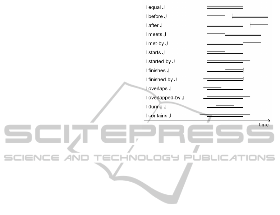
Figure 1: A linear visualization of Allen’s relationships.
Time interval I is visualized here as a grey line segment,
time interval J as a black line segment.
a framework describing such temporal relationships
between time (domain) intervals. Figure 1 visualizes
the temporal relationships Allen discerned.
3 UNCERTAINTY IN TIME
DOMAIN INTERVALS
3.1 Uncertainty and Possibility Theory
Different causes for uncertainty exist. Among oth-
ers, uncertainty about the outcome of an experiment
can be caused by a (partial) lack of knowledge: it
could be known that only one outcome may occur,
but as the experiment is not perfectly and comprehen-
sively known or controlled, the outcome of the exper-
iment may be unknown and thus uncertain. Confi-
dence in the context of uncertainty caused by a (par-
tial) lack of knowledge is modeled using possibility
theory, where possibility is interpreted as plausibil-
ity, given all available knowledge (Bronselaer et al.,
2013).
Based on prior experiences, it is the belief of the
authors that uncertainty concerning time is usually
caused by a (partial) lack of knowledge. Therefore,
the work presented in this paper only considers un-
certainty caused by a (partial) lack of knowledge and
uses possibility theory to model confidence in this
context. In this paper, possibility is always interpreted
as plausibility, given all available knowledge.
TwodimensionalVisualizationofDiscreteTimeDomainIntervalsSubjecttoUncertainty
139

3.2 Ill-known (Time Domain) Intervals
The work presented in this paper will allow time do-
main intervals to be subject to uncertainty by allowing
them to be ill-known time domain intervals. Before
this concept can be explained, the concept of possi-
bilistic variables should be introduced.
Definition 7. Possibilistic Variable (Bronselaer
et al., 2013)
A Possibilistic variable X on a universe Ω is a
variable taking exactly one value in Ω, but for which
this value is unknown. The possibility distribution π
X
on Ω, associated with X, models the available know-
ledge about the value that X takes: for each u ∈ Ω,
π
X
(u) represents the possibility that X takes the value
u.
When a possibilistic variable is defined on a uni-
verse containing intervals, it defines and describes an
ill-known interval (Billiet et al., 2012), (Billiet et al.,
2013b), (Billiet et al., 2013a):
Definition 8. Ill-known Interval (Billiet et al.,
2012), (Billiet et al., 2013b), (Billiet et al., 2013a)
Consider a totally ordered set S containing sin-
gle, atomic values and its powerset ℘(S). Consider
the subset ℘
I
(S) of ℘(S) and let ℘
I
(S) contain every
element of ℘(S) that is an interval, but no other el-
ements. Now consider a possibilistic variable X
˜
I
on
℘
I
(S). The unique, exact value X
˜
I
takes, which is
unknown and which is an interval containing single
values of S, is called an ill-known interval in the pre-
sented work. Seen as the ill-known interval defines
and describes an interval in S, it is also called an ill-
known interval in S.
The interpretation is that an ill-known interval in a
set S represents a specific, precise interval in S which
is unknown. To clarify the difference, an interval not
subject to any imperfection (including uncertainty)
will be called a regular interval in this paper. In the
presented work, ill-known intervals will be denoted
using upper case letters, with a ‘tilde’-sign on top,
e.g.:
˜
I.
The presented proposal will consider ill-known
time domain intervals.
Definition 9. Ill-known Time Domain Interval
An ill-known subset of a time domain of a time
model is called an ill-known time domain interval.
4 TIME DOMAIN INTERVAL
VISUALIZATION
The Triangular Model (TM) comprises a set of rules
indicating how to visualize intervals as points in an
image plane (Kulpa, 2006), (Van De Weghe et al.,
2007). In this section, an adaptation of this technique,
which is used in the presented work, is presented.
Consider a time domain E. The determination of
the point visualizing a time domain interval I ⊆ E us-
ing the TM is illustrated in figure 2. The lower half
of this figure contains a traditional linear visualiza-
tion of I = [t
s
,t
e
] ⊆ E. The upper half of the figure
contains a visualization of I ⊆ E using the TM. In or-
der to accomplish this visualization, first, an interval
in E should be chosen so that its starting element lies
before the starting element of I and its ending ele-
ment lies after the ending element of I. This chosen
interval is visualized as a horizontal straight line seg-
ment in the image plane (Qiang and et al., 2010), (Van
De Weghe et al., 2007), accommodated with vertical
ticks, which visualize the elements of E. This interval
is called the reference interval. In figure 2, it is given
the denotation ‘E’. To visualize I = [t
s
,t
e
] ⊆ E in an
image plane equipped with a visualization of this ref-
erence interval, first the locations of both t
s
and t
e
on
the line segment representing the reference interval
are determined. Next, a straight half-line L
s
is drawn
on the image plane, its initial point being the afore-
mentioned location point of t
s
and another straight
half-line L
e
is drawn on the image plane, its initial
point being the aforementioned location point of t
e
.
These two half-lines are drawn in such a way that they
intersect in a point p and that the size α of the angle
formed by L
s
and the line segment bounded by the lo-
cation points oft
s
andt
e
on the line segment represent-
ing the reference interval is exactly the same as the
size of the angle formed by L
e
and the same line seg-
ment (Qiang and et al., 2010), (Van De Weghe et al.,
2007). This point p is called the interval point (Qiang
and et al., 2010), (Van De Weghe et al., 2007) and the
size α is traditionally chosen to be 45
◦
.
5 VISUALIZING ILL-KNOWN
TIME DOMAIN INTERVALS
In this section, a construction method is described,
which can be used to visualize ill-known time domain
intervals as collections of points in an image plane.
This method is illustrated in figure 3.
Consider a totally ordered time domain E, exactly
as constructed in section 2.2, and its powerset ℘(E).
Consider the subset℘
I
(E) of℘(E) and let℘
I
(E) con-
tain every element of ℘(E) that is an interval, but no
other elements. Now consider an arbitrary ill-known
interval
˜
I ⊆ E, defined by possibilistic variable X
˜
I
on
℘
I
(E), which is defined by possibility distribution π
X
˜
I
on℘
I
(E).
FCTA2014-InternationalConferenceonFuzzyComputationTheoryandApplications
140

linear visualization visualization using the TMlinear visualization
E
E
t
s
t
e
I
I
t
s
t
e
L
s
L
e
Figure 2: The visualization of an interval in time domain E
using the TM and the construction leading to it.
In order to accomplish the visualization of
˜
I, first,
a reference interval is chosen so that its starting ele-
ment lies before every element desired to be visual-
ized and its ending element lies after every element
desired to be visualized. Now, to visualize
˜
I in an
image plane equipped with such a visualization of
this reference interval, the following steps need to be
taken:
1. Consider the subset℘
I
(E) of℘(E).
2. A set I
˜
I
should be constructed, where I
˜
I
contains
all regular intervals K ⊆ E for which π
X
˜
I
(K) > 0
and only these intervals.
3. For every interval K in I
˜
I
fully visualizable in the
figure, the interval point of K is drawn in the im-
age plane following the TM visualization tech-
nique explained in section 4. However, the gray
scale color intensity of the interval point of an in-
tervalK in I
˜
I
now visualizes the possibility π
X
˜
I
(K)
of K of being the interval intended by
˜
I.
The visualization of
˜
I is now the collection of the
visualizations of all the intervals in I
˜
I
. Visualizations
of different intervals may use different colors.
visualization using the TM
E
Possibility 1
Possibility 0
Figure 3: The visualization of an ill-known interval in time
domain E using the TM and the construction leading to it.
Table 1: Allen Relationships corresponding to a DURZ.
Name Allen Relationships
B { before }
BM { before , meets }
BMS { before , meets , starts }
BMO { before , meets , overlaps }
BMOS { before , meets , overlaps , starts }
BMOSD { before , meets , overlaps , starts , during }
BMSD { before , meets , starts , during }
MO { meets , overlaps }
MOS { meets , overlaps , starts }
MOSD { meets , overlaps , starts , during }
MSD { meets , starts , during }
O { overlaps }
OS { overlaps , starts }
OSD { overlaps , starts , during }
SD { starts , during }
D { during }
OF-B { overlaps , finished-by }
DF { during , finishes }
DFM-B { during , finishes , met-by }
OF-BC { overlaps , finished-by , contains }
E { equals }
DFO-B { during , finishes , overlapped-by }
DFO-BM-B { during , finishes , overlapped-by , met-by }
DFO-BM-BA { during , finishes , overlapped-by , met-by , after }
DFM-BA { during , finishes , met-by , after }
F-BC { finished-by , contains }
FO-B { finishes , overlapped-by }
FO-BM-B { finishes , overlapped-by , met-by }
FO-BM-BA { finishes , overlapped-by , met-by , after }
FM-BA { finishes , met-by , after }
C { contains }
CS-B { contains , started-by }
CS-BO-B { contains , started-by }, overlapped-by }
S-BO-B { started-by }, overlapped-by }
O-B { overlapped-by }
O-BM-B { overlapped-by , met-by }
O-BM-BA { overlapped-by , met-by , after }
M-BA { met-by , after }
A { after }
6 DISCRETE UNCERTAIN
RELATIONAL ZONES
In this section, the concept of Discrete Uncertain Re-
lational Zones (DURZ) will be presented.
Consider a totally ordered time domain E, exactly
as constructed in section 2.2. Now consider an arbi-
trary ill-known interval
˜
I ⊆ E and an image contain-
ing a visualization of
˜
I using the construction method
presented in section 5. It is now possible to discern 39
different collections of points in the image plane, de-
pendent on the visualization of
˜
I. Each collection cor-
responds to a single set of Allen relationships. These
collections of points are called
˜
I’s Discrete Uncer-
tain Relational Zones (DURZ). They are related to the
‘Uncertain Relational Zones’ introduced in (De Tr´e
and et al., 2012), but massively expand upon them.
Their visualizations are shown in figures ?? and ?? in
the appendix. In these figures, each collection is given
a unique acronym name. DURZ will be referred to
in this paper using these acronyms. Table 1 shows,
for each DURZ, the unique set of Allen relationships
which corresponds to the DURZ.
Given a totally ordered time domain E, exactly as
constructed in section 2.2, an arbitrary ill-known in-
TwodimensionalVisualizationofDiscreteTimeDomainIntervalsSubjecttoUncertainty
141

terval
˜
I ⊆ E and a visualization of
˜
I using the con-
struction method presented in section 5,
˜
I’s DURZ
in the image containing
˜
I’s visualization can be con-
structed as follows.
Consider the visualizations of the earliest and lat-
est starting and ending points of regular intervals in
E with non-zero possibilities of being the interval in-
tended by
˜
I. For each of these visualizations, draw
two straight half-lines starting in the visualization
point and havingangles with size α with the visualiza-
tion of the reference interval, but with different orien-
tations. Every collection of points now created by an
intersection of these lines, line segments between in-
tersections of these lines and area’s bounded by these
line segments and intersections is now a DURZ, in-
cluding the visualization of
˜
I itself.
The interpretation of such DURZ is the following.
Every intervalpoint in a givenDURZ visualizes a reg-
ular interval in E which has a non-zero possibility of
being in one of the Allen relationships corresponding
to the DURZ, with the interval intended by
˜
I.
7 TEMPORAL RELATIONSHIPS
BETWEEN AN ILL-KNOWN
AND A REGULAR TIME
DOMAIN INTERVAL
In this section, a technique is presented, which allows
to determine, for each existing Allen relationship, the
possibility with which an arbitrary regular time do-
main interval is in this Allen relationship with a given
ill-known interval in the same time domain.
Consider a totally ordered time domain E, exactly
as constructed in section 2.2. Now consider an arbi-
trary regular interval J = [t
s
,t
e
] ⊆ E and a given ill-
known interval
˜
I in E. Now consider the visualization
of
˜
I using the technique described in section 5, its
DURZ and the visualization of J using the TM mo-
del, all in the same image. Now, let the interval point
of J be part of DURZ Z, which corresponds to the
set {R
i
|(0 ≤ i ≤ n) ∧ (i ∈ N)} of Allen relationships,
where every R
i
, 0 ≤ i ≤ n∧i ∈ N is an Allen relation-
ship. For every R
i
, 0 ≤ i ≤ n ∧ i ∈ N, the possibility
π
JR
i
˜
I
with which J is in Allen relationship R
i
with
˜
I is now found visually after the following construc-
tion.
1. The two straight half-lines L
s
and L
e
used to con-
struct J’s interval point are drawn. L
s
’s initial
point is t
s
and L
e
’s initial point is t
e
.
2. Two more straight half-lines L
′
s
and L
′
e
are drawn.
L
′
s
has as initial point t
s
and is orthogonal to L
s
. L
′
e
has as initial point t
e
and is orthogonal to L
e
.
E
L
e
s
Z
s
Figure 4: The evaluation of the temporal relationships be-
tween a regular time domain interval J and an ill-known
time domain interval
˜
I, where J is part of DURZ ‘O’.
3. If none of the half-lines L
s
, L
′
s
, L
e
or L
′
e
contain
any point in the visualization of
˜
I, then Z corre-
sponds to a singleton of Allen Relationships {R
0
}.
In this case, π
JR
0
˜
I
= 1, because J is in Allen
relationship R
0
with
˜
I, regardless of which regular
interval
˜
I is intended to be. An example of this sit-
uation is shown in figure 4. If one or more of the
half-lines L
s
, L
′
s
, L
e
or L
′
e
contain any point in the
visualization of
˜
I, these will divide the collection
of points which is the visualization of
˜
I in as many
sub-collections SC
i
, (0 ≤ i ≤ n) ∧ (i ∈ N) as there
are Allen relationships in the set corresponding to
Z. For this, any set of points of
˜
I’s visualization
all contained by the same half-line L
s
, L
′
s
, L
e
or
L
′
e
is also counted as a sub-collection. In fact,
every sub-collection SC
i
, 0 ≤ i ≤ n ∧ i ∈ N cor-
responds to a single Allen relationship R
i
in this
set: the sub-collection SC
i
contains every point
sc
i, j
, 0 ≤ j ≤ m
i
∧ j ∈ N, where m
i
is the amount
of points in SC
i
, for which J is in this Allen rela-
tionship R
i
with the regular interval having sc
i, j
as
interval point.
4. For every R
i
, 0 ≤ i ≤ n ∧ i ∈ N, it is now easy to
determine π(JR
i
˜
I):
π
JR
i
˜
I
= sup
sc
i, j
∈SC
i
(π
˜
I
(sc
i, j
))
Here, π
˜
I
(sc
i, j
) is the possibility that sc
i, j
is the inter-
val point of the regular interval intended by
˜
I. An
example of this situation is shown in figure 5.
8 TEMPORAL RELATIONSHIPS
BETWEEN TWO ILL-KNOWN
TIME DOMAIN INTERVALS
In this section, a technique is presented, which allows
to determine, for each existing Allen relationship, the
possibility with which an arbitrary ill-known time do-
FCTA2014-InternationalConferenceonFuzzyComputationTheoryandApplications
142
main interval is in this Allen relationship with a given
ill-known interval in the same time domain.
Consider a totally ordered time domain E, exactly
as constructed in section 2.2. Now consider an arbi-
trary ill-known interval
˜
J in E and a given ill-known
interval
˜
I in E. Now consider an image containing
the visualizations of
˜
I and
˜
J and the DURZ of
˜
I. Two
possibilities may be discerned:
• The visualization of
˜
J is completely contained in
a single DURZ corresponding to a singleton of
Allen relationships {R
0
}. In this case, indepen-
dent of which regular interval
˜
J is intended to be
and independent of which regular interval
˜
I is in-
tended to be, the possibility π
˜
JR
0
˜
I
that
˜
J is in
Allen relationship R
0
with
˜
I is 1. This is because
every regular interval with a non-zero possibility
of being the regular interval intended by
˜
J is in
Allen relationship R
0
with every regular interval
with a non-zero possibility of being the regular in-
terval intended by
˜
I. An example of this situation
is shown in figure 6.
• The visualization of
˜
J either is completely con-
tained in a single DURZ corresponding to a set
{R
i,0
|(0 ≤ i ≤ n)∧(i ∈ N)} of Allen relationships,
where every R
i,0
, 0 ≤ i ≤ n∧i ∈ N is an Allen rela-
tionship, or the visualization of
˜
J is partially con-
tained in different DURZ Z
j
corresponding to sets
{R
i, j
|(0 ≤ i ≤ n) ∧ (0 ≤ j ≤ m) ∧ (i ∈ N) ∧ ( j ∈
N)} of Allen relationships, where every R
i, j
, 0 ≤
i ≤ n∧ 0 ≤ j ≤ m∧ 0 ≤ j ≤ n∧i ∈ N ∧ j ∈ N is an
Allen relationship. In these cases, the possibility
π
˜
JR
i, j
˜
I
that
˜
J is in Allen relationship R
i, j
with
˜
I is given by:
π
˜
JR
i, j
˜
I
= sup
∀J∈
˜
J
min
π
˜
J
(J) , π
JR
i, j
˜
I
Here, all J are arbitrary interval points in
˜
J and
π
˜
J
(J) is the possibility that the regular interval in-
tended by
˜
J is J. The formula above illustrates
that for every regular interval J considered, both
E
Ĩ
L
e
s
Z
s
0
1
Figure 5: The evaluation of the temporal relationships be-
tween a regular time domain interval J and an ill-known
time domain interval
˜
I, where J is part of DURZ ‘BMO’.
E
Ĩ
L
e
s
Z
s
Figure 6: The evaluation of the temporal relationships be-
tween ill-known time domain intervals
˜
J and
˜
I, where
˜
J is
part of DURZ ‘O’.
E
Ĩ
L
e
s
s
Figure 7: The evaluation of the temporal relationships be-
tween ill-known time domain intervals
˜
J and
˜
I, where
˜
J is
completely part of DURZ ‘BMO’.
E
Ĩ
L
e
s
s
Figure 8: The evaluation of the temporal relationships be-
tween ill-known time domain intervals
˜
J and
˜
I, where
˜
J is
partially part of DURZ ‘BMO’, ‘MO’ and ‘O’.
the possibility that J is intended by
˜
J and the pos-
sibility that J is in the Allen relationship with
˜
I
should be accounted for. This conjunction is mo-
deled by using the minimum-operator. Examples
of these situations are shown in figures 7 and 8.
9 CONCLUSIONS AND FUTURE
WORK
In this paper, a novel method is presented to visualize
and temporally reason with ill-known time domain in-
tervals. This method is specifically designed for time
TwodimensionalVisualizationofDiscreteTimeDomainIntervalsSubjecttoUncertainty
143

domain intervals and accounts for graded confidence
in the context of uncertainty. Based on the belief that
the source of uncertainty in time usually is a (partial)
lack of knowledge, possibility theory is used to model
confidence. Future work is expected to focus on ad-
vanced querying of such temporal data, using the in-
troduced novel methods for temporal reasoning, and
eventually on data mining in the context of such tem-
poral data.
REFERENCES
Aigner, W. and et al. (2005). PlanningLines: Novel Glyphs
for Representing Temporal Uncertainties and their
Evaluation. In Proc. of the 9th Int. Conf. on Infor-
mation Visualisation, pages 457–463.
Allen, J. (1983). Maintaining knowledge about temporal
intervals. Communications of the ACM, 26:832–843.
Allen, J. F. (1991). Time and time again: The many ways
to represent time. International Journal of Intelligent
Systems, 6(4):341–355.
Billiet, C., Pons, J. E., Pons Capote, O., and De Tr´e, G.
(2012). Evaluating Possibilistic Valid-Time Queries.
In Proceedings of the 14th International Conference
IPMU, Part I, pages 410–419, Catania, Italy. Springer.
Billiet, C., Pons Frias, J. E., Pons, O., and De Tr´e, G.
(2013a). Bipolarity in the Querying of Temporal
Databases, pages 21–37. SRI PAS/IBS PAN, new
trends edition.
Billiet, C., Pons Frias, J. E., Pons Capote, O., and De Tr´e,
G. (2013b). Bipolar Querying of Valid-Time Intervals
Subject to Uncertainty. In Lecture Notes in Computer
Science, pages 401–412, Granada, Spain. Springer.
Bolour, A., Anderson, T. L., Dekeyser, L. J., and Wong, H.
K. T. (1982). The role of time in information process-
ing: a survey. ACM SIGMOD Record, 12:27–50.
Bronselaer, A., Pons, J. E., De Tr´e, G., and Pons, O. (2013).
Possibilistic evaluation of sets. International Journal
of Uncertainty, Fuzziness and Knowledge-Based Sys-
tems, 21(3):325–346.
De Tr´e, G. and et al. (2012). Visualising and Handling Un-
certain Time Intervals in a Two-dimensional Triangu-
lar Space. In Proceedings of the 2nd World Confer-
ence on Soft Computing, pages 585–592, Baku, Azer-
baijan.
Dyreson, C. and et al. (1994). A consensus glossary of tem-
poral database concepts. SIGMOD Rec., 23:52–64.
Dyreson, C. E. and Snodgrass, R. T. (1998). Support-
ing Valid-Time Indeterminacy. ACM Transactions on
Database Systems, 23(1):1–57.
Galton, A. (1990). A Critical Examination of Allen’s The-
ory of Action and Time. Artificial Intelligence, 42(2-
3):159–188.
Garrido, C., Marin, N., and Pons, O. (2009). Fuzzy inter-
vals to represent fuzzy valid time in a temporal rela-
tional database. International Journal of Uncertainty,
Fuzziness and Knowlege-Based Systems, 17(SUPPL.
1):173–192.
Jensen, C. and et al. (1998). The consensus glossary of tem-
poral database concepts - Feb/ 1998 version. In Lec-
ture Notes in Computer Science, pages 367–405.
Kincaid, R. and Lam, H. (2006). Line Graph Ex-
plorer: Scalable Display of Line Graphs Using Fo-
cus+Context. In Proceedings of the Working Confer-
ence on Advanced Visual Interfaces, pages 404–411.
Kulpa, Z. (2006). A diagrammatic approach to investigate
interval relations. Journal of Visual Languages and
Computing.
Matkovic, K. and et al. (2007). Color Lines View: An
Approach to Visualization of Families of Function
Graphs. In Proceedings of the 11th International Con-
ference on Information Visualization, pages 59–64.
Pons, J. E. and et al. (2012). A Relational Model for the Pos-
sibilistic Valid-time Approach. International Journal
of Computational Intelligence Systems, 5(6):1068–
1088.
Qiang, Y. and et al. (2010). Handling imperfect time inter-
vals in a two-dimensional space. Control and Cyber-
netics, 39(4):983–1010.
Qiang, Y. and et al. (2012). Interactive analysis of time
intervals in a two-dimensional space. Information Vi-
sualization.
Saito, T., Miyamura, H. N., Yamamoto, M., Saito, H.,
Hoshiya, Y., and Kaseda, T. (2005). Two-tone pseudo
coloring: Compact visualization for one-dimensional
data. In Proceedings of the IEEE Symposium on In-
formation Visualization, pages 173–180.
Van De Weghe, N., Docter, R., De Maeyer, P., Bechtold, B.,
and Ryckbosch, K. (2007). The triangular model as
an instrument for visualising and analysing residual-
ity. Journal of Archaeological Science.
FCTA2014-InternationalConferenceonFuzzyComputationTheoryandApplications
144

APPENDIX
(a) DURZ ‘B’ (b) DURZ ‘BM’. (c) DURZ ‘BMS’. (d) DURZ ‘BMO’. (e) DURZ ‘BMOS’.
(f) DURZ ‘BMOSD’. (g) DURZ ‘BMSD’. (h) DURZ ‘MO’. (i) DURZ ‘MOS’. (j) DURZ ‘MOSD’.
(k) DURZ ‘MSD’. (l) DURZ ‘O’. (m) DURZ ‘OS’. (n) DURZ ‘OSD’. (o) DURZ ‘SD’.
(p) DURZ ‘D’. (q) DURZ ‘OF-B’. (r) DURZ ‘DF’. (s) DURZ ‘DFM-B’.
Figure 9: The First 19 Collections of Points in the Image Plane Corresponding to the DURZ in a Visualization of the Ill-
Known Interval Ĩ.
(a) DURZ ‘OF-BC’. (b) DURZ ‘E’.Ĩ (c) DURZ ‘DFO-B’. (d) DURZ ‘DFO-BMB’. (e) DURZ ‘DFO-BM-BA’.
(f) DURZ ‘DFM-BA’. (g) DURZ ‘F-BC’. (h) DURZ ‘FO-B’. (i) DURZ ‘FO-BM-B’. (j) DURZ ‘FO-BM-BA’.
(k) DURZ ‘FM-BA’. (l) DURZ ‘C’. (m) DURZ ‘CS-B’. (n) DURZ ‘CS-BO-B’. (o) DURZ ‘S-BO-B’.
(p) DURZ ‘O-B’. (q) DURZ ‘O-BM-B’. (r) DURZ ‘O-BM-BA’. (s) DURZ ‘M-BA’. (t) DURZ ‘A’.
Figure 10: The following 20 collections of points in the image plane corresponding to the DURZ in a visualization of the
ill-known interval Ĩ.
E
Ĩ
E
Ĩ
E
Ĩ
E
Ĩ
E
Ĩ
E
Ĩ
E
Ĩ
E
Ĩ
E
Ĩ
E
Ĩ
E
Ĩ
E
Ĩ
E
Ĩ
E
Ĩ
E
Ĩ
E
Ĩ
E
Ĩ
E
Ĩ
E
Ĩ
E
Ĩ
E E
Ĩ
E
Ĩ
E
Ĩ
E
Ĩ
E
Ĩ
E
Ĩ
E
Ĩ
E
Ĩ
E
Ĩ
E
Ĩ
E
Ĩ
E
Ĩ
E
Ĩ
E
Ĩ
E
Ĩ
E
Ĩ
E
Ĩ
E
Ĩ
TwodimensionalVisualizationofDiscreteTimeDomainIntervalsSubjecttoUncertainty
145
