
Numerical Investigation of Newton’s Method for Solving
Continuous-time Algebraic Riccati Equations
Vasile Sima
1
and Peter Benner
2
1
Advanced Research, National Institute for Research & Development in Informatics,
Bd. Mares¸al Averescu, Nr. 8–10, Bucharest, Romania
2
Max Planck Institute for Dynamics of Complex Technical Systems, Sandtorstraße 1, 39106 Magdeburg, Germany
Keywords:
Algebraic Riccati Equation, Numerical Methods, Optimal Control, Optimal Estimation.
Abstract:
Refined algorithms for solving continuous-time algebraic Riccati equations using Newton’s method with or
without line search are discussed. Their main properties are briefly presented. Algorithmic details incorpo-
rated in the developed solver are described. The results of an extensive performance investigation on a large
collection of examples are summarized. Several numerical difficulties and observed unexpected behavior are
reported. These algorithms are strongly recommended for improving the solutions computed by other solvers.
1 INTRODUCTION
Let A, E ∈ R
n×n
, B, L ∈ R
n×m
, Q and R be symmetric,
Q = Q
T
∈ R
n×n
, R = R
T
∈ R
m×m
, and E and R as-
sumed nonsingular. The generalized continuous-time
algebraic Riccati equations (AREs), or CAREs, with
unknown X = X
T
∈ R
n×n
, are defined by
0 = Q+ op(A)
T
X op(E) + op(E)
T
X op(A)
−L(X)R
−1
L(X)
T
=: R (X), (1)
with
L(X):=L+ op(E)
T
XB.
The operator op(M) represents either M or M
T
. De-
fine also G := BR
−1
B
T
. The numerical solution of
algebraic Riccati equations is required in many com-
putational methods for model reduction, filtering, and
controller design for linear control systems (Lancaster
and Rodman, 1995; Sima, 1996; Bini et al., 2012). An
optimal regulator problem involves the solution of an
ARE with op(M) = M; an optimal estimator problem
involves the solution of an ARE with op(M) = M
T
,
input matrix B replaced by the transpose of the output
matrix C ∈ R
p×n
, and m replaced by p. The solutions
of an ARE arethe matrices X = X
T
for which R (X) =
0. Usually, what is needed is a stabilizing solution, X
s
,
for which the matrix pair (op(A−BK(X
s
)), op(E)) is
stable (i.e., all eigenvalues have strictly negative real
parts), where op(K(X
s
)) is the gain matrix of the op-
timal regulator or estimator, and
K(X) := R
−1
L(X)
T
(2)
(with X replaced by X
s
).
The literature concerning AREs and their use is
overwhelming; see, e.g., the monographs (Anderson
and Moore, 1971; Mehrmann, 1991; Lancaster and
Rodman, 1995; Bini et al., 2012) for many theoreti-
cal results. Numerous numerical methods have been
proposed, and several often-used software implemen-
tations are available, e.g., in MATLAB (MATLAB,
2011), or in the SLICOT Library.
1
Newton’s method
for solving AREs, often attributed to Kleinman, has
been considered by many authors, see, e.g., (Klein-
man, 1968; Mehrmann, 1991; Lancaster and Rodman,
1995; Sima, 1996; Benner and Byers, 1998) and the
references therein. Despite of all these efforts, our
opinion is that its implementation may still be im-
proved. This involves deep investigation and com-
parative analysis of numerical properties and perfor-
mance on large collections of relevant and significant
examples of systems. This paper intends to follow
such an endeavor, based on the results obtained on the
COMPl
e
ib collection (Leibfritz and Lipinski, 2003).
While good performance is already offered by some
software tools, this investigation revealed that further
improvements might still be possible. Moreover, ex-
amples were found for which the expected behavior
has not been observed. These examples have been
further analyzed to find the underlying reasons, and
cures for improving the behavior.
The paper makes use of a refined Newton solver
1
www.slicot.org
404
Sima V. and Benner P..
Numerical Investigation of Newton’s Method for Solving Continuous-time Algebraic Riccati Equations.
DOI: 10.5220/0005117004040409
In Proceedings of the 11th International Conference on Informatics in Control, Automation and Robotics (ICINCO-2014), pages 404-409
ISBN: 978-989-758-039-0
Copyright
c
2014 SCITEPRESS (Science and Technology Publications, Lda.)

with or without line search, and compares its perfor-
mance against the state-of-the-art commercial solver
care
from MATLAB Control System Toolbox. The
MATLAB solver uses an eigenvalue approach, based
on the results in, e.g., (Laub, 1979; Van Dooren,
1981; Arnold and Laub, 1984). One drawback of the
Newton’s method is its dependence on an initializa-
tion, X
0
. This X
0
should be stabilizing, i.e., (op(A −
BK(X
0
)), op(E)) should be stable, if a stabilizing so-
lution X
s
is desired. Except for stable systems, finding
a suitable initialization can be a difficult task. Sta-
bilizing algorithms have been proposed, mainly for
standard systems, e.g., in (Varga, 1981; Hammarling,
1982). However, often such algorithms produce a
matrix X
0
and/or the following several matrices X
k
,
k = 1,2, . . . (computed by Newton’s method), with
very large norms, and the solver may encounter se-
vere numerical difficulties. For this reason, Newton’s
method is best used for iterative improvement of a so-
lution or as defect correction method (Mehrmann and
Tan, 1988), delivering the maximal possible accuracy
when starting from a good approximate solution.
The organization of the paper is as follows. Sec-
tion 2 starts by summarizing the basic theory and
Newton’s algorithms for CAREs. A new formula
for the ratio of successive residuals is given. Sec-
tion 3 presents the main results of an extensive per-
formance investigation of the solvers based on New-
ton’s method, in comparison with the MATLAB
solver
care
. Systems from the COMPl
e
ib collec-
tion (Leibfritz and Lipinski, 2003) are considered.
Section 4 summarizes the conclusions.
2 NEWTON’S ALGORITHMS
The following assumptions are made:
• The matrix E is nonsingular.
• Matrix pair (op(E)
−1
op(A), op(E)
−1
B) is stabi-
lizable.
• The matrix R = R
T
is positive definite (R > 0).
• A stabilizing solution X
s
exists and it is unique.
The conceptual algorithm can be stated as follows:
Algorithm mN: modified Newton’s method, with
line search, for CARE
Input: The coefficient matrices E, A, B, Q, R, and L,
and an initial matrix X
0
= X
T
0
.
Output: The approximate solution X
k
of CARE.
FOR k = 0, 1,...,k
max
, DO
1. If convergenceor non-convergenceis detected, re-
turn X
k
and/or a warning or error indicator value.
2. Compute K
k
:= K(X
k
) with (2) and op(A
k
), where
A
k
= A − BK
k
.
3. Solve in N
k
the continuous-time generalized (or
standard, if E = I
n
) Lyapunov equation
op(A
k
)
T
N
k
op(E) + op(E)
T
N
k
op(A
k
) = −R (X
k
).
4. Find a step size t
k
minimizing the squared Frobe-
nius norm of the residual, kR (X
k
+ tN
k
)k
2
F
, with
respect to t.
5. Update X
k+1
= X
k
+ t
k
N
k
.
END
Standard Newton’s algorithm, briefly referred to as
Algorithm sN below, is obtained by taking t
k
= 1 in
Step 4 at each iteration. When the initial matrix X
0
is
far from a Riccati equation solution, Algorithm mN
often outperforms Algorithm sN.
If the assumptions above hold, and X
0
is stabiliz-
ing, then the iterates of the Algorithm sN satisfy (Ben-
ner and Byers, 1998):
(a) All matrices X
k
are stabilizing.
(b) X
s
≤ · · · ≤ X
k+1
≤ X
k
≤ · · · ≤ X
1
.
(c) lim
k→∞
X
k
= X
s
.
(d) Global quadratic convergence: There is a con-
stant γ > 0 such that
kX
k+1
− X
s
k ≤ γkX
k
− X
s
k
2
, k ≥ 1.
If, in addition, (op(E)
−1
op(A), op(E)
−1
B) is stabi-
lizable and t
k
≥ t
L
> 0, for all k ≥ 0, then the iterates
of the Algorithm mN satisfy
(a) All iterates X
k
are stabilizing.
(b) kR (X
k+1
)k
F
≤ kR (X
k
)k
F
and equality holds if
and only if R (X
k
) = 0.
(c) lim
k→∞
R (X
k
) = 0.
(d) lim
k→∞
X
k
= X
s
.
(e) Quadratic convergence in a neighbourhood of X
s
.
(f) lim
k→∞
t
k
= 1.
Therefore, Algorithm mN does not ensure monotonic
convergence of the iterates X
k
in terms of definite-
ness, contrary to Algorithm sN. But Algorithm mN
achieves monotonic convergence of the residuals to 0,
which is not true for Algorithm sN.
We find now a relation between consecutive resid-
uals R (X
k
) for Algorithm sN. For convenience, we
take E = I
n
, L = 0, and op(M) = M. By definition,
R (X
k
) = A
T
X
k
+ X
k
A− X
k
GX
k
+ Q,
−R (X
k
) = A
T
k
N
k
+ N
k
A
k
= A
T
N
k
+ N
k
A− X
k
GN
k
− N
k
GX
k
,
NumericalInvestigationofNewton'sMethodforSolvingContinuous-timeAlgebraicRiccatiEquations
405

where we have used the formulas from Steps 2 and 3
of Algorithm mN. Summing up the two formulas
above, and using X
k+1
from Step 5 with t
k
= 1, we
get
0 = A
T
X
k+1
+X
k+1
A−X
k
GX
k
+Q−X
k
GN
k
−N
k
GX
k
.
(3)
Also, by definition,
R (X
k+1
) = A
T
X
k+1
+ X
k+1
A− X
k+1
GX
k+1
+ Q, (4)
and subtracting (3) from (4), we have
R (X
k+1
) = −N
k
GN
k
. (5)
It follows that
kR (X
k
)k
F
/kR (X
k+1
)k
F
≈ (kN
k−1
k
F
/kN
k
k
F
)
2
. (6)
If Algorithm sN converges, then kN
k
k
F
is a decresing
sequence, so the ratios in (6) should be greater than 1.
The ratio itself may be taken as a measure of the itera-
tive process speed. Larger ratios imply faster conver-
gence. Numerical evidence has shown that in many
cases, when X
0
has a large norm or is far from X
s
,
these ratios are close to 4 in the initial iterations of
the Algorithm sN for k > 1.
Practical algorithms differ in many details from
the conceptual algorithms above. For instance, it is
not always necessary to use the matrix K(X
k
). In-
deed, if the matrix R is enough well-conditioned with
respect to inversion, the original CARE (1), with
op(M) = M, can be re-written in the form
R (X) =
e
Q+
e
A
T
XE + E
T
X
e
A− E
T
XGXE, (7)
where
e
A := A − BR
−1
L
T
,
e
Q := Q− LR
−1
L
T
. (8)
If m < n/2 it is more efficient to use a factorization of
G. Specifically, let R = L
T
c
L
c
, the Cholesky factoriza-
tion of R, with L
c
upper triangular and nonsingular.
Therefore, by definition, G = DD
T
, with D = BL
−1
c
.
Then, A
k
= A − GXE
T
= A− DD
T
XE
T
. This way,
K(X
k
) is no longer needed, and L has been removed
from the formulas. Moreover, the calculations can be
organized so that common expressions can be com-
puted just once, to reduce the computational effort per
iteration. A solver has been developed based on the
principles mentioned above. It can be used for both
continuous- and discrete-time systems.
3 NUMERICAL RESULTS
This section summarizes some results of an exten-
sive performance investigation of the solvers based
on Newton’s method, and reports deviations from the
expected behavior. The numerical results have been
obtained on an Intel Core i7-3820QM portable com-
puter at 2.7 GHz, with 16 GB RAM, with the rel-
ative machine precision ε
M
≈ 2.22 × 10
−16
, using
Windows 7 Professional (Service Pack 1) operating
system (64 bit), Intel Visual Fortran Composer XE
2011 and MATLAB 8.2.0.701 (R2013b). A SLICOT-
based MATLAB executable MEX-function has been
built using MATLAB-provided optimized LAPACK
and BLAS subroutines.
Linear systems from the COMPl
e
ib collec-
tion (Leibfritz and Lipinski, 2003) have been used.
This collection contains 124 standard continuous-
time examples (with E = I
n
), with several variations,
giving a total of 168 problems. All but 17 problems
(for systems of order larger than 2000, with matrices
in sparse format) have been tried. The performance
index matrices have been chosen as Q = I
n
and R = I
m
.
The matrix L was always zero. In a series of tests, we
used X
0
set to a zero matrix, if A is stable; otherwise,
we tried to initialize the Newton solver with a ma-
trix computed using a MATLAB implementation of
the algorithm in (Hammarling, 1982), and when this
algorithm failed to deliver a stabilizing initialization,
we used the solution provided by the MATLAB func-
tion
care
. A zero initialization was used for 44 sta-
ble examples. The stabilization algorithm was tried
on 107 unstable systems, and succeeded for 91 ex-
amples. The function
care
failed to solve the Riccati
equation for example REA4, since it is unstabilizable.
This example has been excluded from our tests.
We tried both standard and modified Newton’s
methods. The modified solver needed more itera-
tions than the standard solver for 10 examples only.
The cumulative number of iterations with the modi-
fied and the standard solver for all 150 examples was
1657 and 2253, respectively. The mean number of
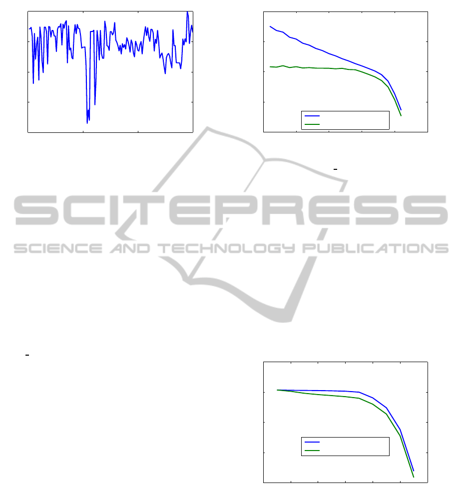
iterations was about 11 and 15, respectively. Fig-
ure 1 plots the ratios between the normalized resid-
uals, k R (X
s
)k
F
/max(1,kX
s
k
F
), obtained by Algo-
rithm sN and those obtained by
care
, when Algo-
rithm sN was initialized by
care
and the tolerance
was set to ε
M
. These ratios indicate the increase in the
solution accuracy (in terms of normalized residuals)
got by Algorithm sN. Using Algorithm mN instead
will not have any advantages with this initialization.
Several situations of unexpected behavior are dis-
cussed in the sequel.
Loss of Stabilization. Having a stabilizing initial-
ization for Newton algorithm is not a guarantee that
the iterates of the Newton process will also be nu-
merically stabilizing. An example was provided by
the COMPl
e
ib system
HF2D9 M256
, with n = 256,
m = 2. Newton process has been initialized by a
ICINCO2014-11thInternationalConferenceonInformaticsinControl,AutomationandRobotics
406
0 50 100 150
10
−8
10
−6
10
−4
10
−2
10
0
Example #
Ratios of residuals
Normalized residual standard Newton/Normalized residual care
Figure 1: Ratios between the normalized residuals found by
standard Newton algorithm and MATLAB
care
for exam-
ples from the COMPl
e
ib collection, using
care
initializa-
tion and tolerance ε
M
.
matrix X
0
generated by the algorithm in (Hammar-
ling, 1982). Since kX
0
k
F
is large, slightly larger than
2.475· 10
13
, the residual R (X
0
) is also very large, al-
though kAk
F
≈ 198.57 and kBk
F
≈ 5.831. Indeed,
kR (X
0
)k
F
≈ 1.166· 10
15
. Consequently, a Lyapunov
solution N
0
with big magnitude, 2.39 · 10
15
, is ob-
tained at iteration k = 0, and the errors propagate to
the next iterations. For Algorithm sN, the closed-
loop matrix at the second iteration becomes unstable.
The iterative process does not converge in 50 itera-
tions, and the instability is inherited. A similar be-
havior resulted also for the Algorithm mN. Although
HF2D9 M256
was the single example witnessing this
difficulty, understanding the reason for the observed
bad behavior was considered of great importance.
The stabilizing algorithm constructs X
0
as the pseudo-
inverse of the solution X
L
of a Lyapunov equation.
That solution has a low-rank, 16, and the computed
X
0
has a large norm. Moreover, the relative residual
of the solution N
0
, based on X
0
, was quite large, about
6 · 10
−4
. But it became 2.7 · 10
−8
when the call to
the MATLAB function
lyap
was replaced by a call
to the SLICOT-based MATLAB function
sllyap
for
computing X
L
. Then, the modified and standard New-
ton’s algorithms converged in 21 and 27 iterations, re-
spectively. Figure 2 shows the nice residual and nor-
malized residual trajectories obtained using the mod-
ified Newton algorithm after changing the initializa-
tion. The behavior remained unchanged for the other
COMPl
e
ib examples after the replacement.
Fast Convergence. To understand why the modi-
fied Newton algorithm can be faster than the stan-
dard Newton algorithm, the behaviour for a simple
COMPl
e
ib example,
AC3
(n = 5, m = 2), will be used.
This is a stable system, hence both Newton algorithms
have been initialized with a zero matrix X
0
. Fig-
0 5 10 15 20 25
10
−20
10
−10
10
0
10
10
10
20
Iteration #
Residuals
Residuals for example HF2D9_M256, modified Newton
Residual
Normalized Residual
Figure 2: Residual and normalized residual trajectories for
COMPl
e
ib example
HF2D9 M256
, using modified Newton
algorithm.
ure 3 and Figure 4 show the residual and normalized
residual trajectories obtained using modified and stan-
dard Newton algorithms, respectively. The use of step
sizes equal to 1 produced a significant increase in the
two residuals at the first iteration (with values about
1.66 · 10
5
and 2.77 · 10
2
). The residuals decrease in
the following iterations, but a larger number of itera-
tions is needed till the iterative process enters into the
region of fast convergencethan for the modified New-
ton algorithm. On the other hand, there is no increase
of residuals in Figure 3. This can happen since the
first Newton steps are smaller than 1. This is a rather
typical behavior.
0 2 4 6 8 10 12
10
−15
10
−10
10
−5
10
0
10
5
Iteration #
Residuals
Residuals for example AC3, modified Newton
Residual
Normalized Residual
Figure 3: Residual and normalized residual trajectories for
COMPl
e
ib example
AC3
, using modified Newton algorithm.
Stagnation. A difficulty with the modified Newton
algorithm is that there might be several consecutive
small step sizes, resulting in a slow convergence. To
avoid this phenomenon, called stagnation, step sizes
of value 1 are used instead of the “optimal” ones. This
corresponds to a reinitialization of the Newton pro-
cess. Such a behavior is illustrated for the COMPl
e
ib
example
AC15
(n = 4, m = 2). Figure 5 shows the
NumericalInvestigationofNewton'sMethodforSolvingContinuous-timeAlgebraicRiccatiEquations
407
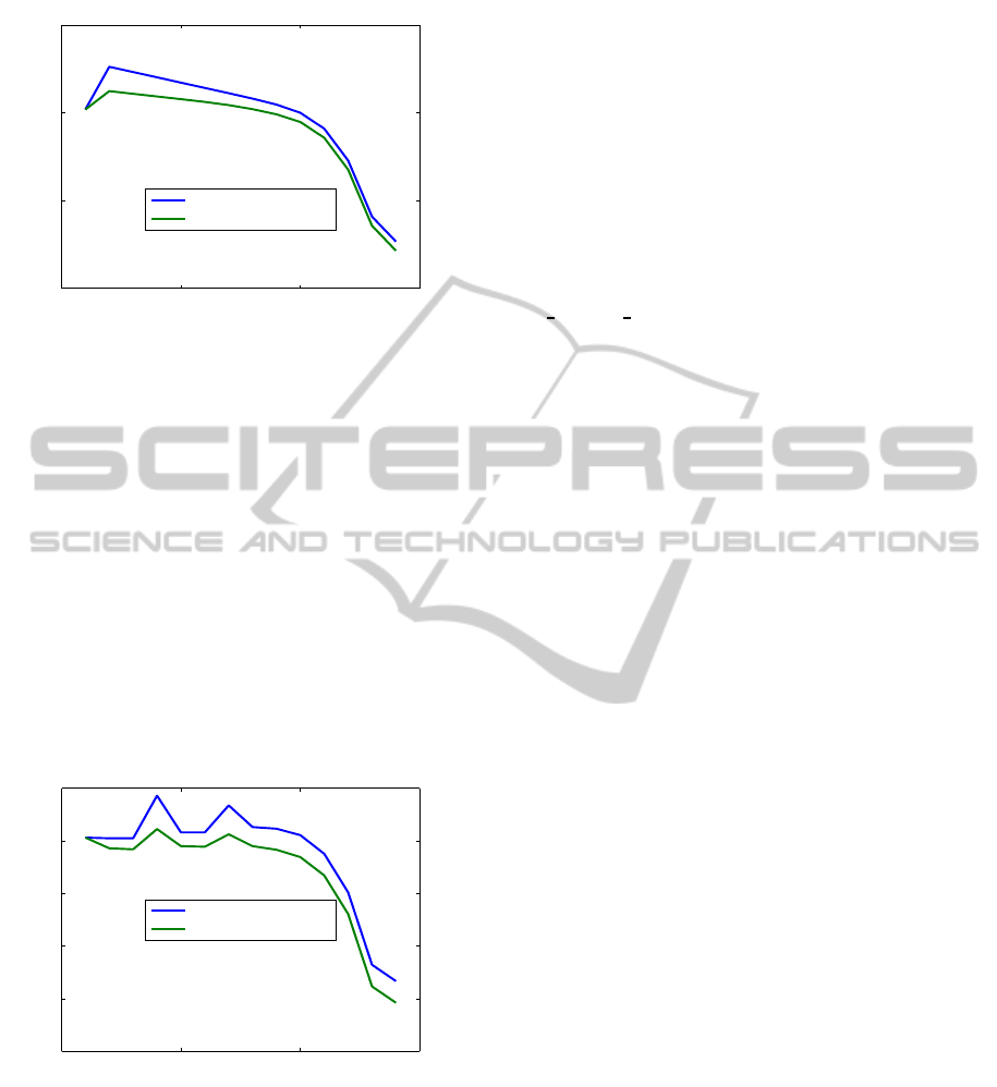
0 5 10 15
10
−20
10
−10
10
0
10
10
Iteration #
Residuals
Residuals for example AC3, standard Newton
Residual
Normalized Residual
Figure 4: Residual and normalized residual trajectories for
COMPl
e
ib example
AC3
, using standard Newton algorithm.
residual and normalized residual trajectories obtained
using the modified Newton algorithm. The first two
step sizes have values about 2.9·10
−4
and 1.17·10
−3
,
and the correspondingresiduals are very close, 1.7315
and 1.7298. The algorithm then uses a step size 1,
which increases the residual to the value 1.94 · 10
4
.
The next iteration takes a step size of about 1.997, re-
ducing the residual to 6.18. The previous behavior is
repeated once more (with different values), but then
the algorithm converges fastly. The standard Newton
algorihm has a smoother behaviour from iteration 1
on (similar to that for example
AC3
in Figure 4), but
it starts with a larger value, 1.19 · 10
7
, and needs one
additional iteration.
0 5 10 15
10
−20
10
−15
10
−10
10
−5
10
0
10
5
Iteration #
Residuals
Residuals for example AC15, modified Newton
Residual
Normalized Residual
Figure 5: Residual and normalized residual trajectories for
COMPl
e
ib example
AC15
, using modified Newton algo-
rithm.
Even if, after setting the step to 1, the modified algo-
rithm produces a residual almost as large as for the
first iteration of the standard Newton algorithm, usu-
ally the next step produces a much lower residual, and
so, the number of iterations decreases. Such a behav-
ior has been seen, e.g., for COMPl
e
ib example
JE1
(n = 30, m = 3), for which, at step 3 of the Newton
algorithm, the residual rose to 3.31·10
10
(from 5.38 at
the previous iteration), but the next residual value was
1.17· 10
4
. The standard algorithm recorded the max-
imal residual of 5.43 · 10
11
at the first iteration. The
number of iterations for convergence were 11 and 17,
respectively.
Slow convergence. The modified Newton algo-
rithm usually converges faster than the standard New-
ton algoritm. However, there are examples for which
the standard algorithm requires less iterations than the
modified algorithm. This happened for COMPl
e
ib
examples
AC5
,
AC18
,
JE2
,
JE3
,
DIS5
,
WEC1
,
NN11
,
CM4 IS
,
CM5 IS
, and
FS
, for which the modified al-
gorithm needed additional 5, 5, 3, 3, 4, 6, 1, 6, 9, and
1 iterations, respectively. To understand the reason
of such a behaviour, consider example
AC18
. Algo-
rithm mN needed 19 iterations, while Algorithm sN
needed only 14. The reason is that Algorithm mN
uses 7 small, comparable steps, but the residual for
all these steps is reduced only by a factor of about
3.5 (from 4.4 · 10
3
to 1.25 · 10
3
). (On the other
hand, using step sizes equal to 1 reduced the resid-
ual faster.) A similar behavior appears for COMPl
e
ib
example
WEC1
, for which Algorithm mN needs 23 it-
erations, while Algorithm sN needs only 17. The
modified algorithm uses 9 small steps (with values in
[0.21,0.33]), but the residual is reduced only with a
factor of about 3 (from 3.1· 10
7
to 1.02 · 10
7
).
This slow convergence is not discovered by the
implemented stagnation detection procedure. A pos-
sible way to improve such a behaviour is to monitor
the succesive reduction factors, defined as ratios be-
tween two consecutive residuals. If the current resid-
ual is high (e.g., higher than 1000) and the mean value
of reduction factors over a certain number of consec-
utive preceding iterations (say, 4) is lower than a cer-
tain value (e.g., 4), then a step size of 1 might improve
the convergence rate. This procedure has not yet been
tried. The rationale for choosing the values above is
as follows. First, such a procedure is not needed when
the residuals are small, since then few iterations will
be sufficient to achieve convergence. Moreover, for
Algorithm mN, the reduction factors may have a large
variation from one iterate to the next one, and there-
fore a moving window of more than two or three iter-
ations is needed to have a useful value for the mean.
Finally, the mean value of 4 is a reasonable selection,
since it was observed that this is the usual value of the
ratios for the initial part of the standard Newton al-
gorithm. Indeed, this was the case for over 90 out of
150 tested COMPl
e
ib examples. Other 30 examples
had ratios larger than 4, while the remaining exam-
ples had either lower values or converged too quickly.
Figure 6 and Figure 7 show the ratios between
ICINCO2014-11thInternationalConferenceonInformaticsinControl,AutomationandRobotics
408
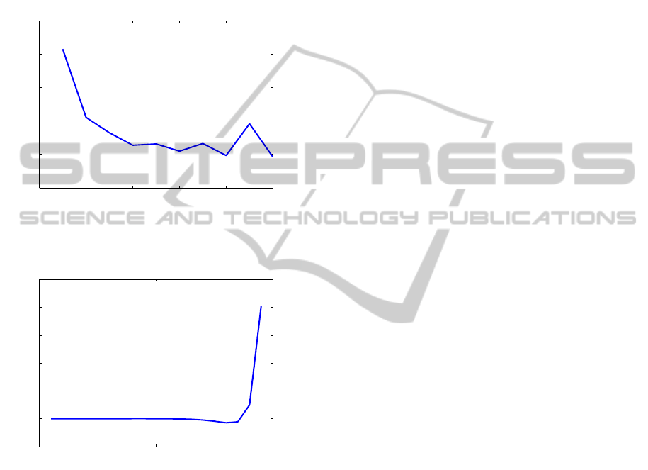
successive residuals for the modified and standard
Newton algorithms for example
AC4
. The ratios have
value 4 for 14 iterations of Algorithm sN. The first ra-
tio, kR (X
1
)k
F
/kR (X
2
)k
F
is not included, since usu-
ally kR (X
2
)k
F
is much larger than kR (X
1
)k
F
, so it
is not relevant for our purposes. Clearly, the modi-
fied Newton algorithm achieves bigger ratios, and so
it converges faster than standard algorithm.
0 2 4 6 8 10
0
5
10
15
20
25
Iteration #
Residual decrease rate
Residual
i
/Residual
i+1
, i=2,... Example AC4, modified Newton
Figure 6: The ratio of successive residuals for COMPl
e
ib
example
AC4
, using modified Newton algorithm.
0 5 10 15 20
3.5
4
4.5
5
5.5
6
6.5
Iteration #
Residual decrease rate
Residual
i
/Residual
i+1
, i=2,... Example AC4, standard Newton
Figure 7: The ratio of successive residuals for COMPl
e
ib
example
AC4
, using standard Newton algorithm.
4 CONCLUSIONS
Basic theory and improved algorithms for solving
continuous-time algebraic Riccati equations using
Newton’s method with or without line search have
been presented. The usefulness of such solvers
is demonstrated by the results of an extensive per-
formance investigation of their numerical behavior,
in comparison with the results obtained using the
widely-used MATLAB function
care
. Systems from
the large COMPl
e
ib collection are considered. The
numerical results most often show significantly im-
proved accuracy (measured in terms of normalized
and relative residuals), and greater efficiency. The re-
sults strongly recommend the use of such algorithms,
especially for improving, with little additional com-
puting effort, the solutions computed by other solvers.
REFERENCES
Anderson, B. D. O. and Moore, J. B. (1971). Linear
Optimal Control. Prentice-Hall, Englewood Cliffs,
New Jersey.
Arnold, III, W. F. and Laub, A. J. (1984). Generalized
eigenproblem algorithms and software for algebraic
Riccati equations. Proc. IEEE, 72(12):1746–1754.
Benner, P. and Byers, R. (1998). An exact line search
method for solving generalized continuous-time alge-
braic Riccati equations. IEEE Trans. Automat. Contr.,
43(1):101–107.
Bini, D. A., Iannazzo, B., and Meini, B. (2012). Numeri-
cal Solution of Algebraic Riccati Equations. SIAM,
Philadelphia.
Hammarling, S. J. (1982). Newton’s method for solving the
algebraic Riccati equation. NPC Report DIIC 12/82,
National Physics Laboratory, Teddington, U.K.
Kleinman, D. L. (1968). On an iterative technique for Ric-
cati equation computations. IEEE Trans. Automat.
Contr., AC–13:114–115.
Lancaster, P. and Rodman, L. (1995). The Algebraic Riccati
Equation. Oxford University Press, Oxford.
Laub, A. J. (1979). A Schur method for solving algebraic
Riccati equations. IEEE Trans. Automat. Contr., AC–
24(6):913–921.
Leibfritz, F. and Lipinski, W. (2003). Description of the
benchmark examples in COMPl
e
ib. Technical report,
Dep. of Mathematics, University of Trier, Germany.
MATLAB (2011). Control System Toolbox User’s Guide.
Version 9.
Mehrmann, V. (1991). The Autonomous Linear Quadratic
Control Problem. Theory and Numerical Solution
Springer-Verlag, Berlin.
Mehrmann, V. and Tan, E. (1988). Defect correction meth-
ods for the solution of algebraic Riccati equations.
IEEE Trans. Automat. Contr., AC–33(7):695–698.
Sima, V. (1996). Algorithms for Linear-Quadratic Opti-
mization. Marcel Dekker, Inc., New York.
Van Dooren, P. (1981). A generalized eigenvalue approach
for solving Riccati equations. SIAM J. Sci. Stat. Com-
put., 2(2):121–135.
Varga, A. (1981). A Schur method for pole assignment.
IEEE Trans. Automat. Contr., AC–26(2):517–519.
NumericalInvestigationofNewton'sMethodforSolvingContinuous-timeAlgebraicRiccatiEquations
409
