
Classification Models of Emotional Biosignals Evoked While Viewing
Affective Pictures
Lachezar Bozhkov
1
and Petia Georgieva
2
1
Computer Science Department, Technical University of Sofia, 8 St.Kliment Ohridski Boulevard, Sofia 1756, Bulgaria
2
DETI/IEETA, University of Aveiro, 3810-193 Aveiro, Portugal
Keywords: Emotion Valence Recognition, Feature Selection, Event Related Potentials (ERPs).
Abstract: This study aims at finding the relationship between EEG-based biosignals and human emotions. Event
Related Potentials (ERPs) are registered from 21 channels of EEG, while subjects were viewing affective
pictures. 12 temporal features (amplitudes and latencies) were offline computed and used as descriptors of
positive and negative emotional states across multiple subjects (inter-subject setting). In this paper we
compare two discriminative approaches : i) a classification model based on all features of one channel and
ii) a classification model based on one features over all channels. The results show that the occipital
channels (for the first classification model) and the latency features (for the second classification model)
have better discriminative capacity achieving 80% and 75% classification accuracy, respectively, for test
data.
1 INTRODUCTION
The quantification and automatic detection of human
emotions is the focus of the interdisciplinary
research field of Affective Computing (AC). In
(Calvo, 2010) a broad overview of the current AC
systems is provided. Major modalities for affect
detection are facial expressions, voice, text, body
language and posture. However, it is easier to fake
facial expressions, posture or change tone of speech
than trying to conceal physiological signals such as
Galvanic Skin Response (GSR) Electrocardiogram
(ECG) or Electroencephalogram (EEG). Since
emotions are known to be related with neural
activity in certain brain areas, affective neuroscience
(AN) emerged as a new modality that attempt to find
the neural correlates of emotional processes
(Dalgleish et al., 2009). The major brain imaging
techniques include EEG, magnetoencephalography
(MEG), functional magnetic resonance imaging
(fMRI) and positron emission tomography (PET).
Among them the EEG modality (Olofsson et al,
2008), (Alzoubi et al., 2009), (Petrantonakis et al.,
2010) has attracted more attention because it is a
noninvasive, relatively cheap and easy to apply
technology. A comprehensive list of EEG-based
emotion recognition researches is recently provided
in (Jatupaiboon , 2013). Despite the first promising
results of the affective neuroscience to decode
human emotional states, a confident neural model of
emotions is still not defined. In our previous works,
we have proposed classification (Bozhkov, 2014)
and clusterisation (Georgieva, 2014) models of
human affective states based on Event Related
Potentials (ERPs) that outperformed other published
outcomes (Jatupaiboon , 2013) . ERPs are transient
components in the EEG generated in response to a
stimulus (a visual or auditory stimulus, for example).
In (Bozhkov, 2014) we studied six supervised
machine learning (ML) algorithms, namely Artificial
Neural Networks (ANN), Logistic Regression
(LogReg), Linear Discriminant Analysis (LDA), k-
Nearest Neighbours (kNN), Naïve Bayes (NB),
Support Vector Machines (SVM), Decision Trees
(DT) and Decision Tree Bootstrap Aggregation
(Tbagger) to distinguish affective valences encoded
into the ERPs collected while subjects were viewing
high arousal images with positive or negative
emotional content. Our work is also inspired by
advances in experimental psychology (Santos,
2008), (Pourtois, 2004) that show a clear relation
between ERPs and visual stimuli with underlined
negative content (images with fearful and disgusted
faces). A crucial step preceding the classification
process was to discover which spatial-temporal
601
Bozhkov L. and Georgieva P..
Classification Models of Emotional Biosignals Evoked While Viewing Affective Pictures.
DOI: 10.5220/0005104206010606
In Proceedings of the 4th International Conference on Simulation and Modeling Methodologies, Technologies and Applications (SIMULTECH-2014),
pages 601-606
ISBN: 978-989-758-038-3
Copyright
c
2014 SCITEPRESS (Science and Technology Publications, Lda.)
patterns (features) in the ERPs indicate that a subject
is exposed to stimuli that induce emotions. We
applied successfully the Sequential Feature Selection
(SFS) technique to minimize significantly the
number of the relevant spatial temporal patterns.
Finally we constructed voting ensemble bucket of
models to take the prediction among all the models
which resulted in very promising final data
discrimination (98%).
In this paper we go further and study the
discriminative priority of the spatial features (which
channel has the highest classification rate) and the
same for the temporal features (which amplitude or
latency of the ERP has the highest classification
rate).
The paper is organized as follows. In section 2
we briefly describe the data set. The ML feature
selection and classification methods used in this
study are summarized in section 3. The results of the
classification model based on all features of one
channel and the classification model based on one
features over all channels are presented in section 4.
Finally, in section 5 our conclusions are drawn.
2 DATA SET
A total of 26 female volunteers participated in the
study, 21 channels of EEG, positioned according to
the 10-20 system and 2 EOG channels (vertical and
horizontal) were sampled at 1000Hz and stored. The
signals were recorded while the volunteers were
viewing pictures selected from the International
Affective Picture System. A total of 24 of high
arousal (> 6) images with positive valence (7.29 +/-
0.65) and negative valence (1.47 +/- 0.24) were
selected. Each image was presented 3 times in a
pseudo-random order and each trial lasted 3500ms:
during the first 750ms, a fixation cross was
presented, then one of the images during 500ms and
at last a black screen during the 2250ms.
The signals were pre-processed (filtered, eye-
movement corrected, baseline compensation and
epoched using NeuroScan. The single-trial signal
length is 950ms with 150ms before the stimulus
onset. The ensemble average for each condition was
also computed and filtered using a zero-phase
filtering scheme. The maximum and minimum
values of the ensemble average signals were
detected. Then starting by the localization of the first
minimum the features are defined as the latency and
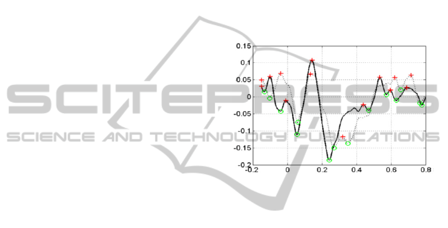
amplitude of the consecutive minimums and the
consecutive maximums (see Fig.1): minimums
(A
min1
, A
min2
, A
min3
), the first three maximums
(A
max1
, A
max2
, A
max3
), and their associated latencies
(L
min1
, L
min2
, L
min3
, L
max1
, L
max2
, L
max3
). The ensemble
average for each condition (positive/negative
valence) was also computed and filtered using a
Butterworth filter of 4th order with passband [0.5 -
15]Hz. The number of features stored per channel is
12 corresponding to the latency (time of occurrence)
and amplitude of either n = 3 maximums and
minimums, the features correspond to the time and
amplitude characteristics of the first three minimums
occurring after T = 0s and the corresponding
maximums in between. The total number of features
per trail is 252.
Figure 1: Extracted features from averaged ERPs: positive
(line) and negative (dot) valence conditions.
3 METHODOLOGY
The feature space consists of 252 features (21
channels x12 features) and the trial examples are 52
(2 classes – positive and negative - for 26 people).
We want to estimate which spatial features (the
channels) and which temporal features (amplitudes
or latencies) have better discriminative capacity.
Therefore, first we build individual classification
models based on all features from each channel.
Thus, 21 channel by channel classifiers are trained,
each of them provided with 12 features (Table1).
Next we build individual models based on each
temporal feature over all channels (Table 1), that is
12 single feature classifiers are trained.
Prior to the classification, the temporal features
(amplitudes and latencies) over the channels were
normalized to improve the learning process. Due to
the relatively small number of training examples,
leave-one-out technique is used for cross validation.
We applied a hierarchical classification approach.
Namely, we first trained the following individual
classifiers: Linear Discriminant Analysis (LDA), k-
Nearest Neighbours (kNN), Naïve Bayes (NB),
SIMULTECH2014-4thInternationalConferenceonSimulationandModelingMethodologies,Technologiesand
Applications
602

Support Vector Machines (SVM) and Decision
Trees (DT). Then, the final classification is based on
the majority of votes between the above classifiers.
Table 1: Channels and Features.
# EEG Channels Feature name
1 Ch 1 (FP1) Amin1
2 Ch 2 (FPz) Amax1
3 Ch 3 (FP2) Amin2
4 Ch 4 (F7) Amax2
5 Ch 5 (F3) Amin3
6 Ch 6 (Fz) Amax3
7 Ch 7 (F4) Lmin1
8 Ch 8 (F8) Lmax1
9 Ch 9 (T7) Lmin2
10 Ch 10 (C3) Lmax2
11 Ch 11 (Cz) Lmin3
12 Ch 12 (C4) Lmax3
13 Ch 13 (T8)
14 Ch 14 (P7)
15 Ch 15 (P3)
16 Ch 16 (Pz)
17 Ch 17 (P4)
18 Ch 18 (P8)
19 Ch 19 (O1)
20 Ch 20 (Oz)
21 Ch 21 (O2)
3.1 Features Normalization
Feature normalization is a typical pre-processing
step in data mining. It usually improves the
classification, particularly when the range of the
features is dispersed. The normalized data is
obtained by subtracting the mean value of each
feature from the original data set and divided by the
standard deviation of the corresponding feature.
Hence, the normalized data has zero mean and
standard deviation equal to 1.
3.2 Leave-One-out Cross-Validation
(LOOCV)
Leave-one-out is the degenerate case of K-Fold
Cross Validation, where K is chosen as the total
number of examples. For a dataset with N examples,
perform N experiments. For each experiment use N-
1 examples for training and the remaining 1 example
for testing [9]. In our case N = 26 (pairs of classes
per person). We will train the models with 25 people
x 2 classes (50 examples) and test on the left-out 2
classes. We are more interested in the total
prediction accuracy for each model, therefore the
predictions are accumulated in confusion matrices
for each model from each training experiment in the
LOOCV.
3.3 Linear Discriminant Analysis
(LDA)
Discriminant analysis is a classification method. It
assumes that different classes generate data based on
different Gaussian distributions. To train (create) a
classifier, the fitting function estimates the
parameters of a Gaussian distribution for each class.
To predict the classes of new data, the trained
classifier finds the class with the smallest
misclassification cost. LDA is also known as the
Fisher discriminant, named for its inventor, Sir R. A.
Fisher [12].
3.4 K-Nearest Neighbour (kNN)
Given a set X of n points and a distance function,
kNN searches for the k closest points in X to a query
point or set of points Y. The kNN search technique
and kNN-based algorithms are widely used as
benchmark learning rules. The relative simplicity of
the kNN search technique makes it easy to compare
the results from other classification techniques to
kNN results. The distance measure is Euclidean.
3.5 Naive Bayes (NB)
The NB classifier is designed for use when features
are independent of one another within each class, but
it appears to work well in practice even when that
independence assumption is not valid. It classifies
data in two steps:
Training step: Using the training samples, the
method estimates the parameters of a probability
distribution, assuming features are conditionally
independent given the class.
Prediction step: For any unseen test sample, the
method computes the posterior probability of that
sample belonging to each class. The method then
classifies the test sample according the largest
posterior probability.
The class-conditional independence assumption
greatly simplifies the training step since you can
estimate the one-dimensional class-conditional
density for each feature individually. While the
class-conditional independence between features is
not true in general, research shows that this
optimistic assumption works well in practice. This
assumption of class independence allows the NB
classifier to better estimate the parameters required
for accurate classification while using less training
data than many other classifiers. This makes it
ClassificationModelsofEmotionalBiosignalsEvokedWhileViewingAffectivePictures
603
particularly effective for datasets containing many
predictors or features.
3.6 Support Vector Machine (SVM)
An SVM classifies data by finding the best
hyperplane that separates all data points of one class
from those of the other class. The best hyperplane
for an SVM means the one with the largest margin
between the two classes. Margin means the maximal
width of the slab parallel to the hyperplane that has
no interior data points. We use radial basis function
for kernel function.
3.7 Decision Tree (DT)
Classification trees and regression trees are the two
main DT techniques to predict responses to data. To
predict a response, follow the decisions in the tree
from the root (beginning) node down to a leaf node.
The leaf node contains the response. Classification
trees give responses that are nominal, such as 'true'
or 'false'.
4 INTER-SUBJECT
CLASSIFICATION MODELS
In this section we summarise the outcomes of the
two classification approaches. The results depicted
in the figures and the tables come from the majority
votes between the five classifiers (LDA, kNN, NB,
SVM and DT).
4.1 Classification Models based on All
Features of a Single Channel
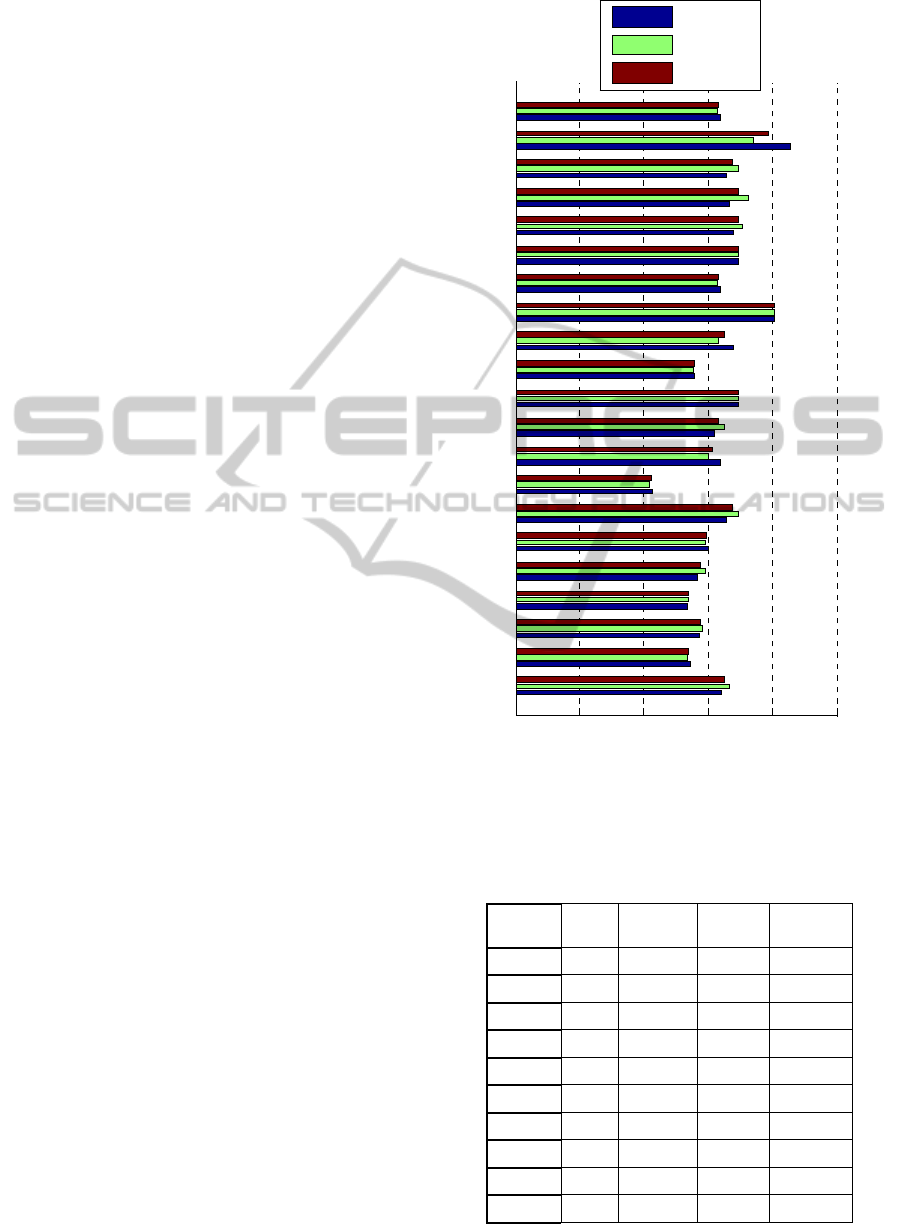
In Figure 2 are given the prediction accuracy results
from each separate channel. In Table 2 are presented
the ordered results including true negative, true
positive and total accuracy by channel. Note that the
discrimination capacity of the occipital and parietal
channels is higher. Hence, the twelve temporal
features associated with these channels are better
descriptors of the two emotional states across 26
persons in our data base. Classification based on all
temporal features in the brain zone around the
occipital channel Oz or the parietal channel P7,
achieve more than 80% accuracy on test data.
Figure 2: Classification accuracy on test data (single
channel- all features).
Table 2: Classification accuracy on test data (single
channel- all features, short list).
Channel Name
True
Negative
True
Positive
Total
Accuracy
14 P7 80,77 80,77 80,77
20 Oz 85,71 74,19 78,85
11 Cz 69,23 69,23 69,23
16 Pz 69,23 69,23 69,23
17 P4 67,86 70,83 69,23
18 P8 66,67 72,73 69,23
7 F4 65,52 69,57 67,31
19 O1 65,52 69,57 67,31
1 FP1 64,29 66,67 65,38
13 T8 68,18 63,33 65,38
0 20 40 60 80 100
1
2
3
4
5
6
7
8
9
10
11
12
13
14
15
16
17
18
19
20
21
Accuracy [%]
Channel
Negative
Positive
Total
SIMULTECH2014-4thInternationalConferenceonSimulationandModelingMethodologies,Technologiesand
Applications
604
4.2 Classification Models Based on a
Single Feature over All Channels
In Figure 3 are given the prediction accuracy results
from each separate temporal feature over all
channels. In Table 3 are presented the ordered
results including true negative, true positive and
total accuracy by feature. Though the results now are
less discriminative compared with the previous
(channel by channel) approach, the last two temporal
features (L
min3
, L
max3
) are significantly better
descriptors (above 70%) of human emotional states
across multiple subjects.
Table 3: Classification accuracy on test data (single
feature- all channels, short list).
Feature Name
True
Negative
True
Positive
Total
Accuracy
12
Lmax3
72,41 78,26 75,00
10
Lmax2
67,74 76,19 71,15
6
Amax3
68,00 66,67 67,31
1
Amin1
64,00 62,96 63,46
11
Lmin3
62,07 65,22 63,46
Figure 3: Classification accuracy on test data (single
feature- all channels).
4.3 Combining Selected Channels and
Features
Having these results we combined the best channels
(Table 4), the best features (Table 5) and intersection
between the best channels and features and achieved
better accuracy result than using single channel or
feature.
Table 4: Combining best performing channels.
Channels 14, 20 14, 20, 11 14,20,11,16
Accuracy 86,54 75 69,23
Table 5: Combining best performing features.
Features 12, 10 12, 10, 6 12,10,6,1
Accuracy 76,92 80,77 76,92
As seen in Table 4 when combining channels 14
(P7) and 20 (Oz) we reach maximum accuracy of
86.54%, then adding more channels slowly
degenerate accuracy. Similar in feature combining
we reached peak accuracy of 80.77% when
combining the first 3 features (L
max3
, L
max2
and
A
max3
).
Using only these 3 features from channels 14 and
20 we reached accuracy of 80.77%, which is the
same accuracy as when used the 3 features from all
21 channels.
4.4 Discussion of the Results
In this paper, we used supervised ML methods to
predict two human emotions based on 252 features
collected from 21 channels EEG. We wanted to
observe which channels and features separately
provide most of the information needed for
classification. In a previous research (Bozhkov,
2014) we achieved 98% accuracy using sequential
selection among all features and channels and voting
by a bucket of ML methods. In this study we
couldn’t reach that high accuracy, however we
reached 86.54% accuracy using only channels 14
and 20 or 80,77% accuracy using features (L
max3
,
L
max2
and A
max3
). This results are similar and better
than similar studies (Jatupaiboon, 2013). Also our
results are similar to a different study on same data
and unsupervised ML methods (Georgieva, 2014).
They obtained highest accuracy when using the
same channels 20(Oz), 16(Pz), 11(Cz) and 14(P7)
and similar features (biased on the late latency
features).
0 20 40 60 80
1
2
3
4
5
6
7
8
9
10
11
12
Accuracy [%]
Feature
Negative
Positive
Total
ClassificationModelsofEmotionalBiosignalsEvokedWhileViewingAffectivePictures
605

5 CONCLUSIONS
In this paper, we propose an alternative approach to
the challenging problem of human emotion
recognition based on brain data. In contrast to most
of the recognition systems where the best spatial-
temporal features are searched, we consider
separately the selection of spatial features (the
channels) and the selection of temporal features
(amplitudes/latencies) in order to distinguish the
processing of stimuli with positive and negative
emotion valence based on ERPs observations. The
core of the present study is to explore the feasibility
of training cross-subject classifiers to make
predictions across multiple human subjects. The
choice of the occipital/parietal channels (more
particularly channel Oz and P7) or the choice of the
temporal features related with the latencies of the
amplitude peaks over all channel (L
max2
,L
min3
,L
max3
)
has the potential to reduce the inter-subject
variability and improve the learning of
representative models valid across multiple subjects.
However, before making stronger conclusions on
the capacity of i) single channel or ii) single feature
over all channels classification models to decode
emotions, further research is required to answer
more challenging questions such as discrimination
of more than two emotions. In fact this is a valid
question for all reported works on affective
neuroscience (Calvo, 2010), (Hidalgo-Muñoz,
2013), (Hidalgo-Muñoz, 2014). The discrimination
is usually limited to two, three, and maximum four
valence-arousal emotional classes. Interesting
problem is also the human personality classification
based on EEG, for example high versus low neurotic
type of personality.
Also, the number of the participants in the
experiments is important for revealing stable cross
subject features. In the reviewed references the
average number of participants is about 10-15, the
maximum is 32. We need publicly available datasets
to compare different techniques and thus speed up
the progress of affective computing.
ACKNOWLEDGEMENTS
We would like to express thanks to the PsyLab from
Departamento de Educação da UA, and particularly
to Dr. Isabel Santos, for providing the data sets.
REFERENCES
Calvo, R. A. & D’Mello, S. K. (2010). Affect Detection:
An Interdisciplinary Review of Models, Methods, and
their Applications. IEEE Transactions on Affective
Computing, 1(1), 18-37.
T. Dalgleish, B. Dunn and D. Mobbs "Affective
Neuroscience: Past, Present, and Future", Emotion
Rev., vol. 1, pp.355 -368 2009.
J. K. Olofsson, S. Nordin , H. Sequeira and J. Polich
"Affective Picture Processing: An Integrative Review
of ERP Findings", Biological Psychology, vol. 77,
pp.247 -265 2008.
O. AlZoubi, R. A. Calvo and R. H. Stevens
"Classification of EEG for Emotion Recognition: An
Adaptive Approach", Proc. 22nd Australasian Joint
Conf. Artificial Intelligence, pp.52 -61 2009.
P. C. Petrantonakis and L. J. Hadjileontiadis "Emotion
Recognition from EEC Using Higher Order
Crossings", IEEE Trans. Information Technology in
Biomedicine, vol. 14, no. 2, pp.186 -194 2010.
N. Jatupaiboon, S. Panngum, P. Israsena, Real-Time EEG-
Based Happiness Detection System, The
ScientificWorld Journal, Vol. 2013, Article ID 18649,
12 pages.
Santos, I. M., Iglesias, J., Olivares, E. I. & Young, A. W.
(2008). Differential effects of object-based attention
on evoked potentials to fearful and disgusted faces.
Neuropsychologia, 46, 1468-1479.
Pourtois, G., Grandjean, D., Sander, D., & Vuilleumier, P.
(2004). Electrophysiological correlates of rapid spatial
orienting towards fearful faces. Cerebral Cortex,
14(6), 619–633.
Christopher M. Bishop (2006). Pattern Recognition and
Machine Learning. Springer.
Fisher, R. A. The Use of Multiple Measurements in
Taxonomic Problems. Annals of Eugenics, Vol. 7, pp.
179–188, 1936.
O. Georgieva, S. Milanov, P. Georgieva, I.M. Santos,
A.T.Pereira, C. F. da Silva (2014), Learning to decode
human emotions from ERPs, Neural Computing and
Applications, Springer (in press).
Bozhkov L., P. Georgieva, R. Trifonov, Brain Neural Data
Analysis Using Machine Learning Feature Selection
and Classification Methods. 15th Int. Conf. on
Engineering Applications of Neural Networks
(EANN'14) 5-7 Sept. 2014, Sofia, Bulgaria.
(accepted).
A. R. Hidalgo-Muñoz, M. L. Pérez, A. Galvao-Carmona,
A. T. Pereira, I. M. Santos, M. Vázquez-Marrufo, Ana
Maria Tomé. EEG study on affective valence elicited
by novel and familiar pictures using ERD/ERS and
SVM-RFE. Medical & Biological Engineering &
Computing, 52(2), 149-158, 2014.
A. R. Hidalgo-Muñoz, M. L. Pérez, I.M. Santos, A.T.
Pereira, M. Vázquez-Marrufo, A. Galvao-Carmona,
Ana Maria Tomé. Application of SVM-RFE on EEG
signals for detecting the most relevant scalp regions
linked to affective valence processing. Expert Systems
with Applications, 40 (6) , 2102-2108, 2013.
SIMULTECH2014-4thInternationalConferenceonSimulationandModelingMethodologies,Technologiesand
Applications
606
