Parametrical and Procedural Approach in the

LIDAR Data Visualisation

Complex Creation of the Photorealistic and Accurate 3D Model of the Surface

Jan Hovad and Jitka Komarkova

Faculty of Economics and Administration, University of Pardubice, Studentska 84, 532 10 Pardubice, Czech Republic

Keywords: Dtm, Dsm, Lidar, Polygon, 3D Model, Visualisation.

Abstract: Author presents a new hybrid method for LIDAR processing in the form of complex, real-world attribute-

based 3D digital model of the terrain. This model can be widely used for 3D GIS analyses, visualization for

public contracts, construction of new communications (roads), GPS navigation and generating individual

views from any location. Model is based on the LIDAR scanned values that are transferred into the

quadrilateral polygonal form. The main goal is to reconstruct large scale areas in 3D by slope based

quadrilateral grids that are interpolated from irregular raw structure. Laser scan is checked and corrected. It

is simplified by chosen interpolation technique into the quadrilateral set of grids (C++). Each grid has

different resolution to lower hardware requirements. Raw scan is analysed by slope factor and is used

further to classify grids into a groups. Classified grids are processed by 3D scripting language to form

polygonal terrain model. Vector and polygonal data are converted into 3D and utilized to reconstruct surface

features and terrain classes. Set operations are used to divide digital terrain model into the segments. Set of

high polygonal models is created for each class. These models are scattered on the top of the classified

polygonal surface.

1 INTRODUCTION

Light detection and ranging (LIDAR) is frequently

used technology that provides information about

elevation of scanned objects, their position,

classification etc.. This scan is usually obtained by a

special modified airplane or it is combined with

ground LIDAR scanners. Raw data source is formed

by individual points with basic x, y and z attributes.

Scanned area includes all captured points detected

by detection device and it is called Digital Surface

Model (DSM). These points can be segmented and

classified by chosen algorithms. For example the

laser beam reflected only from the terrain, forms

Digital Terrain Model (DTM). Other model type can

include only buildings that form, after extraction

from a DSM, a Digital Building Model (DBM).

Extracted trees form a Digital Canopy Height Model

(DCHM) and so on (Broveli at al. 2004, Omasa et al.

2008, Chen et al. 2012). All these models along with

models from other branches (engineering), can be

unified and merged together.

Creation of DTM is frequently initial activity in

the LIDAR data pre-processing. In the past 20 years

there was the whole set of algorithms to extract the

best representation of DTM (Hu 2003, Elmqvist

2002, Kraus and Pfeifer 2001).

Other categories include prediction of DTM,

accuracy analysis against the real data sets and

simplifying LIDAR point cloud. It is often

impossible to obtain data at all of the points in the

area of interest. Therefore it is necessary to compute

these missing values additionally. Spatial

interpolation calculates an unknown value from a set

of points with known values. For many applied

objectives it is necessary to create a regular square

surface formed from quadrilaterals - in this paper

called quad regular network (QRN). This procedure

can be created using the following local/global

approach of the selected algorithm - Renka-Cline,

Shepard, IDW, etc. (R. J. Renka and A. K. Cline

1984, McLain 1976, Lawson 1977, Akima 1978).

Current applied utilization of DTM creation is

very rich and intersects a wide range of scientific

disciplines. DTM and its hybrid shape forms are

used in Austria by Mandlburger et al. (2009) for

156

Hovad J. and Komarkova J..

Parametrical and Procedural Approach in the LIDAR Data Visualisation - Complex Creation of the Photorealistic and Accurate 3D Model of the Surface.

DOI: 10.5220/0005098001560161

In Proceedings of the 9th International Conference on Software Engineering and Applications (ICSOFT-EA-2014), pages 156-161

ISBN: 978-989-758-036-9

 2014 SCITEPRESS (Science and Technology Publications, Lda.)

analysing terrain models for river flow modelling.

Mandlburger found that the data reduction is

necessary but in other hand it can bring significant

errors. DBM is created by many approaches like

slopes evaluation (Zhou et al. 2004), building

extraction from space borne imagery (Tack at al.

2011) or they were extruded from the DEM

(Priestnall et al. 2000). DBM can be used for GPS

signal prediction. Li et al. (2007) explained a ray

tracing method, which was applied to prediction and

visualization of GPS signal in dense urban areas.

Implementation of a real-time satellite visibility was

also researched by Taylor et al. (2006). Besides GPS

the DBM can be used directly in evaluating the Sun

exposure time in case of constructing the solar

panels on the top of the building roofs. This study

was explained by Nguyen et al. (2012). Scientific

research and applied usage of LIDAR is also

directed into agriculture and forestry.

LIDAR topic is widely discussed but its

applications can be still extended. Each algorithm or

method is usually used for certain purposes like in

urban areas to create DBM. Different results can be

obtained when creating DTM, topographic position

can shift the algorithm precision and so on.

Approach of combining different steps, algorithms

and methods is usually needed to solve a specific

problem. Proposed solution allows direct

interconnection of the geography, architecture,

engineering and transport outputs (simulation,

analyses) together. For example, authors are able to

calculate GIS analyses, import 3D model of the

bridge with calculated stress and tension analysis

from the engineer, integrate building models from

the architect and print everything by the 3D printer

or create photorealistic animations/visualisation of

the output. This kind of approach is described in this

article.

2 GOALS

The main goal is: LIDAR data utilization in case of

reconstructing large scale areas in the 3D by slope

based quadrilateral grids to form photo-realistic

model of the surface, which is based on the real-

world values scanned by laser.

Partial goals are: Laser scan is carefully checked

and corrected - registered, merged, de-noised etc.

Laser scan is simplified by chosen interpolation

technique into the form of quadrilateral set of grids

(C++/Python). Each grid has different resolution to

lower hardware requirements - adaptive approach.

Laser scan is analysed by slopes and this analysis is

used further to classify interpolated grids into

groups. Classified grids are processed by 3D

scripting language to form polygonal quadrilateral

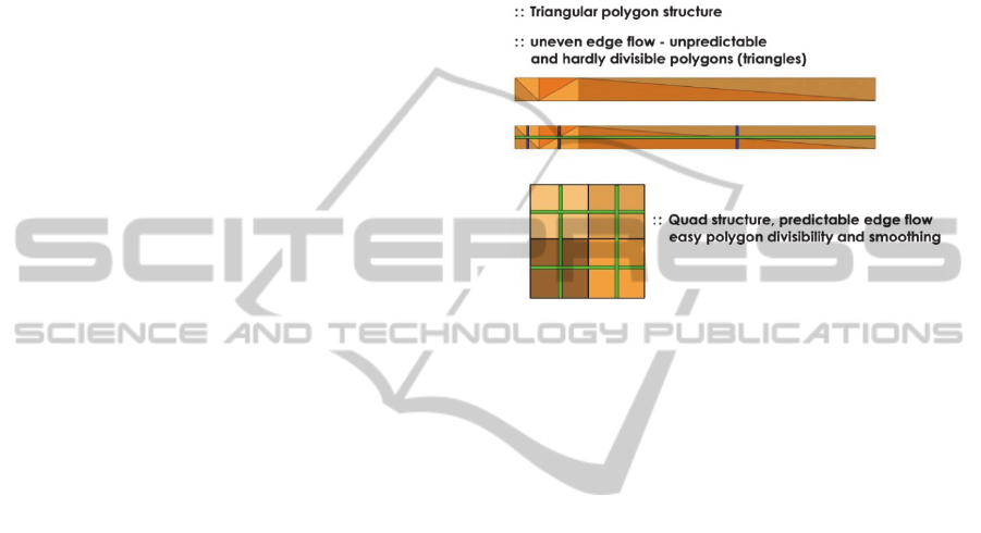
digital terrain model. Points are intersected by

splines predictably and they form a regular shaped

quadrilaterals that can be further divided and

adjusted to match the imported object properties

(Figure 1).

Figure 1: Surface division.

Vector data are converted into 3D and utilized to

reconstruct rivers, roads, buildings and terrain

classes. All other objects can be placed into the

model. Quadrilateral structure allows unlimited

smoothing by intersecting additive splines through

the polygon. Set operations are used to divide digital

terrain model into the classes (forests, fields, urban

areas, water surfaces etc.). A set of high polygonal

models is created for each class. Models are

scattered on the top of the classified surface and the

static outputs are formed (Figure 2).

2.1 Used Data, Software and Hardware

Authors have two data inputs available. LIDAR scan

for the area size roughly 10×20 km. Data set is

scanned by aircraft Turbolet L-410 FG. Outputs

create two types of LIDAR models. First, the Digital

Surface Model 1

Generation (DSM 1G) which

includes all objects on the surface (terrain +

vegetation, buildings…). The second is the Digital

Model of the Relief 5

Generation (DMR 5G)

(Belka 2012). Scanned values are stored as XYZ

coordinates (Figure 3).

Each scanned value is represented by separate

line with information about X/Y coordinate (WGS

1984) and Z elevation attribute (meters above sea

level).

The second data type is vector layer from the

database ZABAGED

, which contains the basic

surface features like rivers, roads, terrain types etc.

ParametricalandProceduralApproachintheLIDARDataVisualisation-ComplexCreationofthePhotorealisticand

Accurate3DModeloftheSurface

157

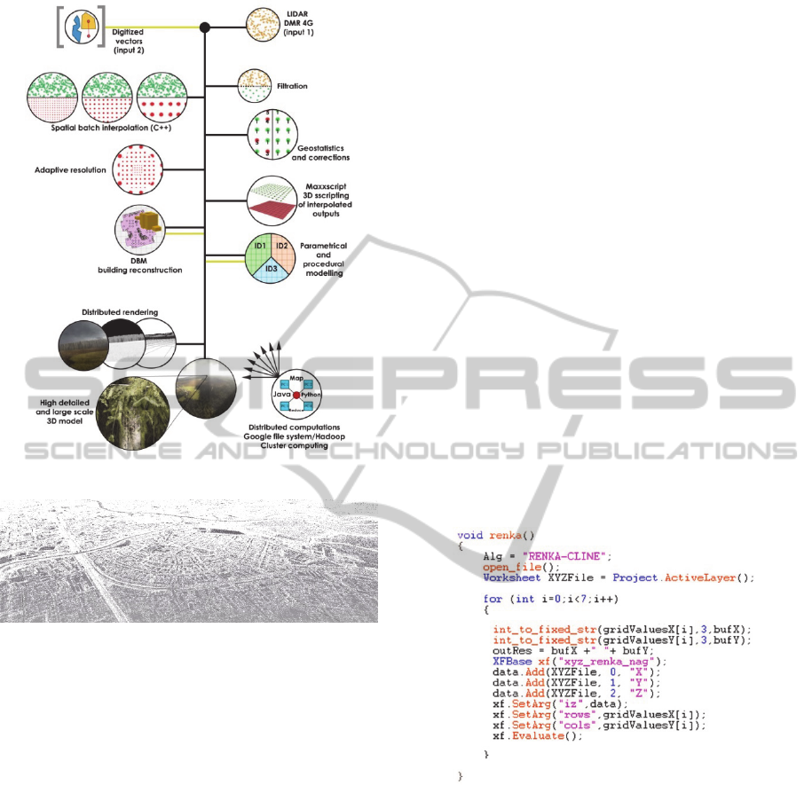
Figure 2: Proposed solution.

Figure 3: LIDAR point cloud.

Hardware requirements are quite moderate

because authors process the big data volumes.

Authors used two computers to perform individual

operations. AMD Opteron and Intel i7 2600K CPU,

with minimum of 16 GB memory, fast SATA III

SSD (500 MB/s) and GeForce 460 GTX. The most

important is high amount of memory to work with a

large number of points. Render farm in Germany is

used as a remote cloud station to get quick static

outputs from the 3D model.

Software that is used is mainly a 64 bit to fully

utilize RAM capacity. It is ArcGIS 10 SP3,

SagaGIS, OriginLab. These applications fully

sufficed in all GIS analyses and allowed

programming the batch interpolation tasks.

Programming can be made with the help of

integrated Python or C++. Authors utilized national

algorithm library (NAG) for C++. Graphical tasks

are completed in the Autodesk 3D Studio Max 2012

and its Maxxscript module that allows object

oriented scripting and processing of wide range of

data inputs.

3 METHODS

This chapter characterizes details of the individual

steps as described in the Figure 2.

3.1 Spatial Interpolation and Adaptive

Approach

This text uses local interpolation of Inverse Distance

Weighting (IDW) and global version of Renka-Cline

interpolation. The whole irregular structure is batch

processed by a C++. The code saves all interpolated

grid outputs into specified folder. Each output is

saved in the different resolution defined by a target

size of required polygon. Target size of polygons is

set to array of {5 10 20 40 60 100} meters.

Computation results in two input arrays that form a

raw empty grid that is filled by interp. values, COLS

{100,167,251,502,1005,2010}, ROWS {199,332,49

8,997,1995,3990}. C++ code solves the batch tasks

of performing Renka-Cline within an application

OriginLab. Source code shows only a few lines of

procedure code due to the limits of the article size

(Figure 4).

Figure 4: Main part of the source code for Renka-Cline

interpolation.

Files with grids are stored in the created

directory. Each of them is compared against slope

analysed DEM and clipped into 3 major groups

based on the National Slope Classification system.

This process creates detailed grids for areas with

sharp elevation changes and low resolution grids for

flat areas. Minor overlaps are apparent and they help

to connect all regions. Hardware requirements are

lowered (Figure 5) (Svobodová 2011).

ICSOFT-EA2014-9thInternationalConferenceonSoftwareEngineeringandApplications

158

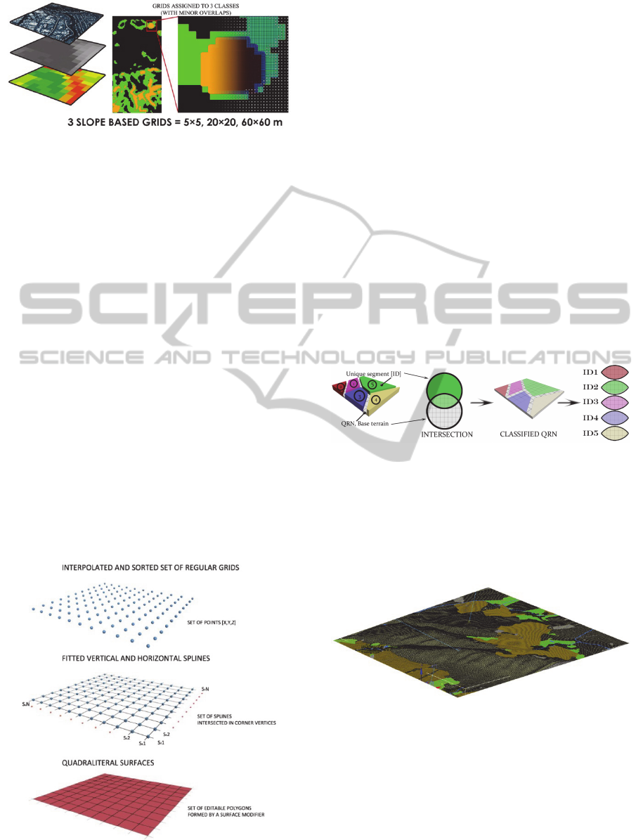
Figure 5: Spatial and adaptive grids.

3.2 3D Scripting of Chosen Point

Inputs

According to the previous step, the set of grids is

chosen. That minimizes the amount of spatial

deviation in the area of interest. This structure is still

represented by a points or optionally raster coded

values. Each set has a different resolution and point

offset. Each row or column (points are interpolated

into predefined grid size already) must be sorted and

intersected by a spline to fit each point in the good

order. This step forms a quadrilateral polygon

structure, where the polygons are equal in the area

size, which means that they can be easily

subdivided. The following procedure can be done in

any 3D environment that supports work with

vectors/polygons and allows the use of scripting or

programming techniques to access the individual

objects within the source code. This requirement is

met for example by the Maxxscript, 3D scripting

language, which is available as the part of the 3D

Studio Max. Full implementation of the principle

can be expressed in the graphical form (Figure 6).

Figure 6: Author´s approach to create point to polygon

surface.

Selected data are loaded from the text files line

by line (point by point). Each array is then sorted

and the line is intersected vertically and horizontally.

Sorting process can be time consuming task (in case

of higher inputs). Authors recommend to pre-

compute this step by distributed approach (Hadoop).

3.3 Parametrical and Procedural

Modelling

In this phase of work, the terrain is formed from

continuous quadrilateral polygonal structure with

houses on the top of the surface. What needs to be

done is to clip the surface into groups, classes. There

are two ways to do this. The first one utilizes

modern LIDAR scanners that handle classification

automatically. This is not the author’s case. The

second option is to use set operations (intersect) and

digitized vectors from publicly available databases.

The process of creating surface ID for each class is

shown in the following picture (Figure 7).

Figure 7: Set operations to create unique terrain segments.

The terrain model is ready to be fitted with

models. Each terrain ID receives a set of adequate

models that are scattered on the top of the surface.

The model for the given area after applied

intersection is shown in Figure 8.

Figure 8: Segmented terrain 3D model.

All work in the visualisation is planned to be

purely parametrical and procedural without any

needs of the subjective interventions. The word

parametrical means that authors prepared for each

ID a set of high-polygonal objects that are suitable

for individual terrain sections. These objects are

modelled separately, which take some time, but they

can be used in the infinitely many projects

repeatedly. Authors are able to exclude this step in

ParametricalandProceduralApproachintheLIDARDataVisualisation-ComplexCreationofthePhotorealisticand

Accurate3DModeloftheSurface

159

the future. Everything can be performed almost

automatically. More models for each ID section

forms better outputs because of variability.

Word procedural is here crucial because every

object material is very simple. Materials are created

only in the procedural way of combining colours.

All the details are stored in the high-polygonal

models that are stored as proxies. Proxies are not

hardware challenging but they are unpacked when

making final render. Memory is saved and GPU,

which influences the speed while working with the

model, is not so busy. FPS (Frame Per Second) is

higher and total operability is increased. The

different colour of models is made by colour map,

which is applied to each section. Each section has a

scattered class assigned, that has multiple properties

used to vary each object from the other one. Main

attributes are distribution (uniform, random),

random/fixed scale/move/rotation, collisions,

normals and many other parameters. These objects

that contain all the scattering information and

reference models can be transferred from one project

to any other. This makes the visualization of ArcGIS

analysis very flexible and time effective. Next very

simplified image shows a few model clusters ready

to be placed and modified on the basis of the

assigned ID. Attributes can be based on the exact

value from LIDAR.

The point structure is very reduced, all the

surface objects are stored as Proxy objects, terrain is

quadrilateral, each polygon contains only 4 points

while the surface is adaptive (higher slopes have

smaller polygons, flatter areas have bigger

polygons). This situation can be illustrated by the

following 3D model output. This is completely

computer generated imagery, not a photograph

(CGI), which is based on the LIDAR point cloud

values. The values are derived into the 3D model ()

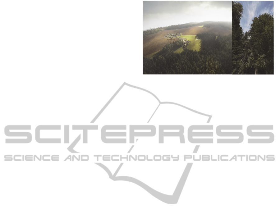
The camera can be placed anywhere in the model

or it can be animated. The general level of detail is

very high even in case of close-ups because the

proxy objects are very detailed. This can be

demonstrated by placing the secondary camera into

the altitude of 550 meters and the third camera into

the middle of the forest below (Figure 9).

4 DISCUSSION AND

CONCLUSION

This section summarizes the results and outlines

possible ways forward in the future research.

Figure 9: Level of detail, random camera placement.

4.1 Discussion

Authors completed all stated goals with success.

However, some tasks can be adjusted and improved.

Therefore, the future work is going to be directed

into the area of a raster driven scattering. Every

model on the surface will be scattered on the basis of

the black-white raster map. This map can store the

LIDAR values like tree height or tree width in much

lower hardware demanding form. There is no need

to use statistical approach while scattering the proxy

objects. Every tree can have an exact position as in

the real world in the time of the scanning.

The second task that can be enhanced is the

digital weather model. In this case, clouds are

generated randomly. In the future work, the NOAA

images are connected with the 3D model. Particle

system is created and clouds are generated in 15

minutes intervals.

4.2 Conclusion

Authors propose a method, which encapsulates

outputs from the GIS analyses, LIDAR data

processing, DBM acquisition and terrain creation to

utilize all these steps in parametrical and procedural

scientific visualization. The resulting 3D model can

be widely used for 3D GIS analyses, visualizations

for public contracts, planning and construction of

new communications (roads, bridges, etc.),

simulations, 3D printing, GPS navigation and

generating individual static/dynamic views from any

location. The result connects GIS with other

sciences like architecture, agriculture, forestry or

road design and can be further used as a GIS server

with large dimensioned 3D terrain model (C# .NET).

Client side can provide user interface to fill

parameters like camera position, target position,

camera settings, weather condition, file formats etc.

The rendered output can be sent to the client.

Studios that must remodel each environment for the

ICSOFT-EA2014-9thInternationalConferenceonSoftwareEngineeringandApplications

160

client manually can lower the costs significantly by

use of already created large scaled model. There are

so many application possibilities that it is hard to

mention all of them.

ACKNOWLEDGEMENTS

This work was supported by the project No.

CZ.1.07/2.2.00/28.032 Innovation and support of

doctoral study program (INDOP), financed from EU

and Czech Republic funds.

REFERENCES

Akima, H., 1978. A method of bivariate interpolation and

smooth surface fitting for irregularly distributed data

points, ACM TOMS, 4, 148-64.

Belka, L., 2012. Airborne laser scanning and production of

the new elevation model in the Czech Republic,

Vojenský geografický obzor, 55 (1), 19-25.

Broveli, M. A., Canata, M. and Longoni, U.M, 2004.

LIDAR data filtering and DTM interpolation within

GRASS, Transactions in GIS, 8(2), 155-174.

Chen, Z., Devereux, B., Gao, B. and Amable, G., 2012.

Upward-fusion urban DTM generating method using

airborne LIDAR data, Journal of Photogrammetry and

Remote Sensing, 72, 121-130.

Elmquist, M., 2002. Ground surface estimation from

airborne laser scanning data with morphological

methods, Photogrammetric Engineering & Remote

Sensing, 73 (2), 175-185.

Hu, Y., 2003, Automated Extraction of Digital Terrain

Models, PhD Thesis. University of Calgary, Canada

Kraus, K. and Pfeifer, N., 2001. Advanced DTM

generation from LIDAR data, International Archives

of Photogrammetry and Remote Sensing, 34(3), 23-30.

Lawson, C. L., 1977. Software for C surface interpolation,

Mathematical Software, 3, 161-194.

Li, J., Taylor G., Kidner, D. and Ware, M., 2008.

Prediction and visualization of GPS multipath signals

in urban areas using LIDAR Digital Surface Models

and building footprints, International Journal of

Geographical Information Science, 22 (11-12), 1197-

1218.

Mandburger, G., Hauer, C., Hofle, B., Habersack, H. and

Pfeifer, N., 2009. Optimization of LIDAR derived

terrain models for river flow modeling, Hydrology and

Earth System Sciences, 1453-1466.

Mclain, D.H., 1976. Two dimensional interpolation from

Random Data, Computer J., 384, 179-181.

Nguyen, H. T., Pearce, J. M., Harrap, R. and Barber, G.,

2012. The Application of LIDAR to Assessment of

Rooftop Solar Photovoltaic Deployment Potential in a

Municipal District Unit, Sensors, 12, 4534-4559.

Omasa, K., Hosoi, F., Uenishi, T. M., Shimizu, Y. and

Akiyama, Y., 2008. Three-Dimensional Modeling of

an Urban Park and Trees by Combined Airborne and

Portable On-Ground Scanning LIDAR, Remote

Sensing, Environmental Modeling & Assessment,

13(4), 473-481.

Priestnall, G., Jaafar, J. and Duncan, A., 2000. Extracting

urban features from LIDAR digital surface models,

Computers, Environmental and Urban Systems, 24,

65-78.

Renka, R. J. and Cline, A. K., 1984. A triangle-based C

Interpolation Method. Journal of Mathematics, 14,

223-237.

Svobodova, J., 2011. Quality assessment of digital

elevation models for environmental applications.,

Thesis, University of Ostrava, 174p, Available in

Czech only: Title: Hodnocení kvality digitálních

výškových modelů pro environmentální aplikace

Tack, F., Buyuksalih, G. and Goossens, R., 2012. 3D

building reconstruction based on given ground plan

information and surface models extracted from

spaceborne imagery, ISPRS Journal of

Photogrammetry and Remote Sensing, 67, 52-64.

Taylor, G., Li, J., Kidner, D., Brunsdon, CH. and Ware,

M., 2007. Modeling and prediction of GPS availability

with digital photogrammetry and LIDAR,

International Journal of Geographical Information

Science, 21 (1), 1-20.

Zhou, G., Song, C., Simmers, J. and CHeng, P., 2004.

Urban 3D GIS From LIDAR and digital aerial images,

Computers & Geosciences, 30, 345-353.

ParametricalandProceduralApproachintheLIDARDataVisualisation-ComplexCreationofthePhotorealisticand

Accurate3DModeloftheSurface

161