
Numerical Backward Simulation Model
with Case Branching Capability
Yukio Hiranaka, Houjin Sakaki, Kenta Ito, Toshihiro Taketa and Shinichi Miura
Department of Informatics, Yamagata University, Yonezawa, Japan
Keywords: Backward Simulation, Numerical Backward Model, Case Branching Simulation, Range Signal.
Abstract: The authors are studying backward simulators which trace from results to causes for comprehensive
verification of system safety. It is not easy to make a backward simulation model because the forward
model may not be expressed in a reversible formula, or it is not reversible in cases of multiple inputs or
inclusion of internal state variables. In this paper, we propose a backward simulator which can incorporate
numerical simulation models and has a case branching capability to deal with multiple inputs. As a practical
simulation target, we implemented a simulator for testing stability of dynamic pricing for power usage
control as a smart grid application. We show some illustrating results of the backward simulation.
1 INTRODUCTION
Securing proper operation of software systems is a
great concern for our IT centric society. Software
engineers are doing their elaborate work to achieve
safety of their system by tests, which cannot be fully
done for almost all the applications. Essential
difficulty in the work comes from the fact that
engineers start their design by a forward thinking for
implementing functions to accomplish the objective
of the system, and they will take in unexpected
situations in their system, unintentionally.
A secure system might be designed by a backward
thinking to use only secure components with a safe
structure by considering all the unfavorable
conditions which may be encountered. However, it
may be a practical way that we design a system in a
forward thinking and check the safety of it by
backward testing. We describe a method for such
check with rounding up failure conditions by a
backward simulator in this paper.
2 BACKWARD SIMULATION
AND TARGET SIMULATION
We describe our backward simulator for a case of
control situation. As a smart power grid application,
dynamic pricing is planned and evaluated for
suppressing electricity consumption (Schweppe et al,
1981, Freeman, 2005,
Mohsenian-Rad 2010, Fan,
2011, Koulsopoulos and Tassiulas, 2011). The idea
is simple enough that consumers will reduce their
usage if the power company raise the price of
electricity. However, some may worry about the
dynamic behaviour of user and price determination.
If many consumers use some kind of automatic cost
cutter or economizing unit, power usage will be
decreased instantly after the price raised or
announced to be lowered and will be increased
instantly after the price lowered or announced to be
raised, and then, oscillation should be observed,
which might be uncontrollable at the worst.
We should investigate full consequences of the
system behaviors. Usually, it is not possible to test
all the conditions that the system would encounter
by using a forward simulator because the cases to be
tested would be huge in number.
There are backward approaches to search a
reasonable solution under certain restrictions such as
a dynamic allocation of resources (Huang et al.,
2009) and fault analysis (FTA). However, there is no
practical backward simulator for detecting
unfavorable conditions without leak.
So, we created a backward simulator to round up
all the unfavorable conditions by defining range
signals (Hiranaka et al., 2012). A range signal
expresses the range of values on control links and it
is used to calculate the possible input signal in the
backward simulation. If we start with unfavorable
output range, we can calculate input range signal
225
Hiranaka Y., Sakaki H., Ito K., Taketa T. and Miura S..
Numerical Backward Simulation Model with Case Branching Capability.
DOI: 10.5220/0005096302250230
In Proceedings of the 4th International Conference on Simulation and Modeling Methodologies, Technologies and Applications (SIMULTECH-2014),
pages 225-230
ISBN: 978-989-758-038-3
Copyright
c
2014 SCITEPRESS (Science and Technology Publications, Lda.)

which covers the condition on which the unfavorable
output occurs. Our aim is to detect such range, to
narrow down the condition and, then, to verify
whether the system would output unfavorable value.
Our backward simulator was implemented by
using Scala Language to use its Actor functions.
Range signals are expressed in XML style data
format (we call it as UCF Universal Communication
Format) which is comprised of the destination part
and the content part. The simulator has forward
simulation functions and distinguishes forward and
backward signal by the destination part of range
signals. If the destination is an input (typically
identified by <i>) of the block, then the content part
will be processed by the forward algorithm. If the
destination is an output (typically identified by <o>),
then the content part will be processed by the
backward algorithm.
It is not an easy task to make a backward
simulator, generally. The difficulties are encountered
to make a backward algorithm for each simulation
component when the forward algorithm is not
expressed in a simple formula, when it has multiple
inputs and when it has inner state variables which
cannot be determined from the output. Our solutions
to such situations are by using numerical inclusive
algorithm, by case branching (Hiranaka et al., 2013)
with dividing the possible conditions into finite
cases of input range pairs, and by externalizing the
inner state variables out of simulation blocks,
respectively. This paper shows the former two
methods.
Fig.1 is the whole view of a simple forward
simulation structure for testing dynamic pricing.
Four blocks represent a pricing block, a room
temperature sensor block, a user response block and
a heater block. The block named as sim is the
simulation controller which can intervene or
advance the simulation sequences by its
coordination function. All the simulation blocks
send their range signal messages to sim and sim
relays them to the predetermined block(s) down the
flow.
i
i
i
t
o
temp
user
heater
price
sim
o
o
Figure 1: Forward simulator example.
Fig.2 shows the backward simulation structure
corresponding to Fig.1, just reversed the direction of
signal flows indicated by dashed lines. The
component manin is a signal injection component
for initiating backward simulation. Along the
backward flow, the value range expressed by the
range signal will gradually become wider because
the backward algorithm needs to be designed to a
safer side, not to leak unfavourable conditions.
i
i
i
t
o
o
o
temp
user
heater
price
manin
sim
Figure 2: Backward simulator corresponding to Fig.1.
3 NUMERICAL FORWARD AND
BACKWARD MODEL
This section describes how the numerical model
blocks are formed. As for a case of electric oil heater
(De’Longhi TDD0915W), we measured switch
position to power usage relation, which is
summarized in Table 1. Then, the forward algorithm
of heater is to output power usage corresponding to
the input switch position (0 to 3). The backward
algorithm is to output the range of switch position
corresponding to the power usage range, e.g. range 1
to 2 switch position in response to 0.5 kW to 1 kW
backward signal. If the incoming power usage range
does not cover any of the values, this component
sends an out of range message to the simulation
controller.
An example of backward range signal from heater
component to user component is
<user><s>delong<s>i</s></s><t>100.0</t><o>1,
2</o><user>
where <s> tag means message source with nested
source i, which means the input port of delong
heater, and <o> tag means the entry point of the
range data “1,2.” The tag <t> means timestamp
indicating output time relative to the forward
simulation start time. It is advanced in forward
simulation and rewound in backward simulation for
the specified value predetermined by each
simulation component.
SIMULTECH2014-4thInternationalConferenceonSimulationandModelingMethodologies,Technologiesand
Applications
226

Table 1: Characteristics of De’Longhi heater.
Switch position power usage(kw)
0 0.0
1 0.58
2 0.83
3 1.39
Forward pricing model was set as in Table 2,
where p is the price (Yen/kWh), u is the total usage
(kW) and C is the supply capacity (kW). It may be
determined by a mathematical formula (such as in
Fan, 2011). Backward model for the price
component (Table 3) is just an exchange of input
and output of Table 2, from which the range of
power usage divided by the capacity is determined
by price value or by range of price values.
Forward user model was set as in Table 4,
representing a user who determines the switch
position of the heater responding to the electricity
price and the selected room temperature. Backward
model for the user component (Table 5) is derived
from Table 4, from which range of room
temperature is determined by the switch position
depending on the electricity price. In this case, we
need to select which price value to be simulated
further. Such selection and proceeding is dealt by
case branching described latter.
Table 2: Forward price model.
u/C P (Yen/kWh)
low high
0 0.5 11
0.5 0.8 22
0.8
∞
44
Table 3: Backward price model.
p (Yen/kWh)
u/C
min max
11 0 0.5
22 0.5 0.8
44 0.8
∞
Table 4: A forward user response model.
room
temperature
p (Yen/kwh)
11 22 44
0 3 3 3
5 3 3 3
10 3 3 2
15 3 2 1
20 2 1 0
25 0 0 0
Table 5: Backward user response model corresponding to
Table 4.
Switch
position
room temperature range
price=11 price=22 price=44
0
22.5 – ∞ 22.5 – ∞ 17.5 – ∞
1 22.5 – 22.5 17.5 – 22.5 12.5 – 17.5
2 17.5 – 22.5 12.5 – 17.5 7.5 – 12.5
3
- ∞– 17.5 - ∞ – 12.5 - ∞ – 7.5
The forward temp component is just send the
current room temperature to the user block. We set it
as constant for the simulation period. Backward
temp model has a special function. It can accept any
valid room temperature range, but it assumes that the
temperature is constant for the simulation period and
do not allow the incoming temperature range to be
outside of the former range, then, gradually
narrowed by successive backward temperature range
signal. If it detects invalid temperature range, it
informs sim that the current case corresponding to
the invalid range signal is not feasible.
4 RANGE VS. RESOLUTION
As stated in the section 2 referring to Fig.2, value
range of range signals are getting wider through the
backward simulation and would spread too much.
However, we can get detailed results by dividing the
range.
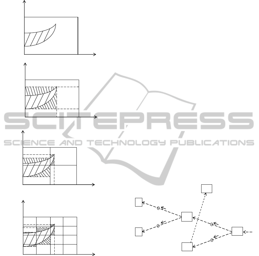
Fig. 3 shows how the division of range signal
affects the simulation resolution, which means the
degree of coincidence between the resultant range
and the true area of unfavorable conditions. In the
figure, (a) shows the true area of unfavorable
conditions, (b) shows the rectangle which is defined
by the range of x and the range of y, (c) shows a
narrowed area defined by a combination of
rectangles for each divided range of x and range of
y. And if we proceed the range division further as in
(d), we will come closer to the true area of question.
Such improvement of resolution can be done by
dividing the temperature range in the user model.
5 CASE BRANCHING CONTROL
In this section, we describe the details of case branch
processing. All the components in the Fig. 2 except
manin deals branch related messages of branch,
clearCase, nextCase, branchCompleted, which are
control messages between simulation components.
A component which needs to branch pushes the
cases to be tested further onto its case stack and
sends a branch signal with a unique branch id to sim.
NumericalBackwardSimulationModelwithCaseBranchingCapability
227
y
x
(a)
a
y
a
x
b
y
b
x
(b)
y
x
1
y
1
x
a
y
a
x
b
y
b
x
(c)
y
x
c
y
1
y
1
x
a
y
a
x
b
y
b
x
(d)
y
x
c
y
2
x
d
y
Figure 3: Range signal division and result resolution.
In the response to it, sim sends a branch signal and a
clearCase signal in sequence, each with the branch
id, to all the components.
Receiving the branch signal, every component
prepares to branch by storing the internal states and
keeps branch id in its local branch id stack.
Receiving the clearCase signal, it resets the internal
state to be the saved status, and sends a ready signal
to sim. Receiving ready signals from all the
components, sim sends a nextCase signal to all the
components. Receiving the nextCase signal, only the
component which generated the branch id coinciding
with the branch id in the nextCase message pops up
a case from its case stack and sends the related range
signal for the selected case backward to the
connected upstream component through sim. Then
sim proceeds simulation for the case selected by the
branch generated component.
If any of the components detects invalid incoming
range signal, it will send nextCase message to sim.
Receiving nextCase message, sim sends a clearCase
message to all the components and return to the state
of waiting ready signals from all the components
before to proceed to the next nextCase. If all the
cases for one branch have been tested, the
component which generated the branch sends a
branchCompleted message to sim with branch id,
and sim sends the branchCompleted message to all
the components. Receiving branchCompleted
message, all the components including sim pop the
branch id stack and prepares to proceed the former
simulation before that branch.
An example of branch message from user to sim
is
<sim><s>user</s><branch>user#1</branch></sim>
where “user#1” is the branch id generated by the
user component. Other messages like clearCase,
nextCase, breanchComplete and ready use the same
format by changing the <branch> tag to a tag of each
message’s name.
<o>1,2</o>
<o>10,20</o>
E
<o>3,4</o>
<o>2,20</o>
X
X
A
B
C
D X
sim
<nextCase>E#1</nextCase>
Figure 4: Invalid signal to stop processing the case.
6 IMPLEMENTATION AND
RESULTS OF OPERATION
Fig. 5 shows GUI windows of simulation
components. Fig.6 shows an example of command
window display. The simulation controller sim has a
step button for stepwise checking. And also, it has a
nextCase button for manually skip the current case
to the next case because we have no algorithm to
stop a branched case which may run forever.
SIMULTECH2014-4thInternationalConferenceonSimulationandModelingMethodologies,Technologiesand
Applications
228
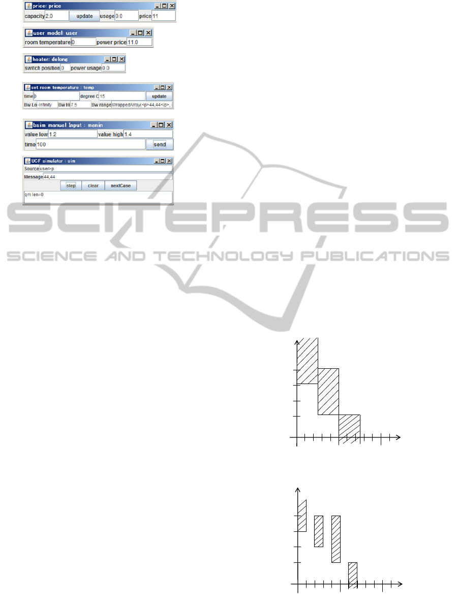
Figure 5: GUI for each simulation component.
$ scala P.P
Iprice started. capacity=2.0
Iuser started. room temperature=0 power price=11.0 Yen/kwh
Idelong started. switch positon=0
Itemp started. time=0 value=15
Imanin started. time=100 low=1.1 high=2.2
Isim started.
Btemp 0 15
Duser 0.0 3
Ddelong 1.0 1.39
Dprice 2.0 22
Duser 7.0 2
Ddelong 8.0 0.83
Dprice 9.0 11
Duser 14.0 3
Ddelong 15.0 1.39
Dprice 16.0 22
Figure 6: Console example of forward simulation.
Fig.7 shows a console display of a backward
simulation. The starting power usage value is
injected manually by using manin component. The
left end shows the type of console message and the
source of the message. At the center, time of
message generation is displayed and it goes
backward. The remaining message shows the range
values and supplemental information.
By injecting a range signal of power usage, e.g.
0 to 0.5kW, backward into the simulator, we can
determine whether the injected range is feasible or
not. If some component detects that incoming range
is not allowed, any value in the injected range
cannot be reached by the system. If the simulation
continues without such detection, it shows that there
is a condition which causes the system to output the
value inside the injected range. In such cases, we can
obtain temperature range for the injected range
because temp component of our implementation
keeps temperature range narrowed by successive
backward range signals.
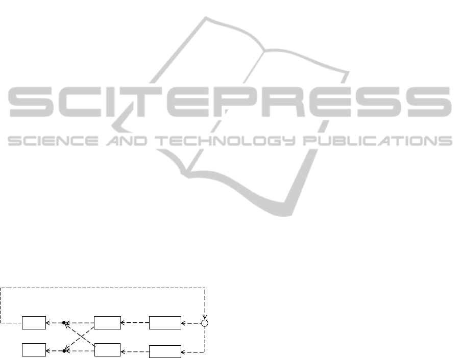
Fig. 8 shows temperature range in relation to
injected power usage range of 0-0.5, 0.5-1.0, 1.0-1.5
or 1.5-2.0, each with 0.5kW interval. The hatched
area means the area of possibility. Fig.9 shows the
same relation in the case of 0.2kW interval. The
hatched area in Fig.9 is within that of Fig.8. It
indicates that we can arbitrary control the resolution
of the result.
Iprice started. capacity=2.0
Iuser started. room temperature=0 power price=11.0 Yen/kwh
Idelong started. switch positon=0
Itemp started. time=0 value=15
Imanin started. time=100 low=1.1 high=2.2
Isim started.
Bmanin 100 1.4,1.6
Wdelong 99.0 input 1.4, 1.6 is out of range 0.0, 1.39
Isim simulation completed.
Bmanin 100 1.2,1.4
Bdelong 99.0 input 3,3 for 1.2,1.4
Buser 94.0 input price=44,44 temp=-Infinity,7.5
Bdelong 92.0 input 2,3 for 0.8,Infinity
Buser 87.0 input price=44,44 temp=-Infinity,12.5
Bdelong 85.0 input 2,3 for 0.8,Infinity
Figure 7: Console example of backward simulation.
1.0
2.0
kw
temp
22.5
17.5
12.5
7.5
0
0
Figure 8: Simulation result for 0.5kW step ranges.
1.0
2.0
kw
temp
22.5
17.5
12.5
7.5
0
0
Figure 9: Simulation result for 0.2kW step ranges.
NumericalBackwardSimulationModelwithCaseBranchingCapability
229
Although the above results are for a simple
simulation model, it was shown that the backward
simulator can catch the unfavorable conditions and
can narrow down the area of such conditions.
To make Figs 8 and 9, we need to judge the
simulation trace displayed in Fig.7 whether it
continues forever or not for the feasible cases.
Probably, we have to set some time limit for each
case’s calculation, beyond which the simulator
automatically judges the case feasible.
7 CONCLUSION AND FUTURE
WORK
We designed the forward and backward simulator
with capability of using numerical simulation
models, backward range processing and case
branching. The implemented simulator shows
validity of the backward simulation for a simple case
of dynamic pricing control model planned for smart
grid.
We need to have many experiences by applying
the simulator to practical applications. Multiple user
simulation (Fig.10) is the top on our list, which
requires multiple branching components and a
backward sum component. We have to estimate
processing time of our backward simulator in the
case of large number of branches. Also, we plan to
design automatic judging algorithm for cases of
continuing or vibrating simulation. And also,
externalization of internal state variables will be
demanded in a complex system simulation.
p
p
i
i
o
o
1
i
o
2
i
i
i
temp
user1
heater1
price
user2
heater2
o
o
o
1
o
+
o
con-p
con-t
2
o
r
r
i
1
o
2
o
Figure 10: A backward simulation structure for two users.
ACKNOWLEDGEMENTS
This work was partly supported by JSPS KAKENHI
Grant Number 25540006. The authors wish to thank
the reviewers for their valuable comments.
REFERENCES
Chen, L., Steven, N.L., Low, H. and Doyle, J., 2010. Two
Market Models for Demand Response in Power
Networks, Proc. IEEE Int’l Conf Smart Grid Comm.
Fan, Z. 2011. Distributed Demand Response and User
Adaptation in Smart Grid, Proc. Integrated Network
Management, pp.726-729.
Freeman, R., 2005. Managing Energy: Reducing Peak
Load and Managing Risk with Demand Response and
Demand Side Management, Refocus, vol.6, no.5,
pp.53-55.
FTA, Fault Tree Analysis, http://en.wikipedia.org/
wiki/Fault_tree_analysis
Hiranaka, Y. and Taketa, T., 2012. Designing Backward
Range Simulator For System Diagnoses, Proc. XX
Imeko World Congress Metrology for Green Growth.
Hiranaka, Y., Taketa, T. and Miura, S., 2013. Case
Branching Backward Simulator for Integer
Factorization, Proc. 8th EUROSIM Congress on
Modeling and Simulation, pp.259-264.
Huang, C.C. and Wang, H.H., 2009. Backward Simulation
with Multiple Objectives Control, Proc. IMECS
(International MultiConference of Engineers and
Computer Scientist).
Koulsopoulos I. and Tassiulas, 2011. L., Challenges in
Demand Load Control for the Smart Grid, IEEE
Network, vol.25,no.5, pp.16-21.
Mohsenian-Rad, A.H., Wong V.W.S., Jatskevich, J.,
Schober, R. and Leon-Garcia A., 2010. Autonomus
Demand-Side Management Based on Game-Theoretic
Energy Consumption Scheduling for the Future Smart
Grid, IEEE trans. Smart Grid, vol.1, no.3, pp.320-331.
Schweppe F.C., Tabors R.D. and Kirtley J.L., 1981.
Homeostatic Control: The Utility/Customer
Marketplace for Electric Power, MIT Energy
Laboratory Report, MIT-EL 81-033.
SIMULTECH2014-4thInternationalConferenceonSimulationandModelingMethodologies,Technologiesand
Applications
230
