
Detailed Modeling and Calibration of a Time-of-Flight Camera
Christoph Hertzberg and Udo Frese
FB3 - Mathematics and Computer Science, University of Bremen, 28359 Bremen, Germany
Keywords:
Time-of-Flight Camera, Depth Sensor, Sensor Model, Calibration, Robustified Corner Extraction, High
Dynamic Range, Lens Scattering.
Abstract:
In this paper we propose a physically motivated sensor model of Time-of-Flight cameras. We provide meth-
ods to calibrate our proposed model and compensate all modeled effects. This enables us to reliably detect
and filter out inconsistent measurements and to record high dynamic range (HDR) images. We believe that
HDR images have a significant benefit especially for mapping narrow-spaced environments as in urban search
and rescue. We provide methods to invert our model in real-time and gain significantly higher precision than
using the vendor-provided sensor driver. In contrast to previously published purely phenomenological calibra-
tion methods our model is physically motivated and thus better captures the structure of the different effects
involved.
1 INTRODUCTION
Time-of-Flight (ToF) cameras are compact sized sen-
sors which provide dense 3D images at high frame
rates. In principle, this makes them advantageous for
robot navigation (Weingarten et al., 2004), iterative
closest point (ICP)-based 3D simultaneous localiza-
tion and mapping (SLAM) (May et al., 2009) and as
a supporting sensor for monocular SLAM (Castaneda
et al., 2011). The advantages come at the cost of many
systematic errors, which, to our knowledge, have not
been systematically analyzed and modeled so far. Es-
pecially for ICP-based SLAM it is crucial to remove
or reduce systematic errors.
With the recent introduction of low-cost structured
light cameras (most famously the Microsoft Kinect)
and the KinectFusion algorithm (Newcombe et al.,
2011) most research has shifted away from ToF cam-
eras. Despite the much more complex systematic
errors of ToF cameras, we still think they have the
important advantages of a more compact size and
the ability to detect finer structures. This is because
structured light sensors cannot detect objects smaller
than the sampling density of the structured light pat-
tern, while ToF cameras can detect even objects of
sub-pixel dimension if their reflectance is high com-
pared to the background. Both are important, e.g.,
in narrow-spaced SLAM scenarios, where we believe
ToF cameras have the potential to supersede struc-
tured light and stereo vision. In this paper, we fo-
cus on the PMD CamBoard nano (PMDtechnologies,
2012), but our results should be transferable to similar
sensors.
In the remainder of the introduction, we recapit-
ulate an idealistic sensor model that is often found
in the literature and list phenomena where the actual
sensor differs from that model. Afterwards, we dis-
cuss related work in Sec. 2, followed by Sections 3
to 6 describing the phenomena and their calibration.
We verify our results and show the impact of the com-
pensation by means of a practical example in Sec. 7
before finishing with an outlook in Sec. 8.
1.1 Idealistic Sensor Model
The general measurement principle of ToF cameras is
to send out a modulated light signal and measure its
amplitude and phase offset as it returns to the camera
(Lange, 2000, §1.3, §2.2), cf. Fig. 1. In the simplest
Figure 1: Idealistic Sensor Model. The LED emits mod-
ulated light which is reflected by the scene on the right
(dashed red paths). From the phase-offset of the received
light the sensor can calculate distances and these can be
used to build a 3D model of the scene (blue dots on the
left). The wave length of the modulation is ideally greater
than the longest path lengths expected in the application.
568
Hertzberg C. and Frese U..
Detailed Modeling and Calibration of a Time-of-Flight Camera.
DOI: 10.5220/0005067205680579
In Proceedings of the 11th International Conference on Informatics in Control, Automation and Robotics (ICINCO-2014), pages 568-579
ISBN: 978-989-758-039-0
Copyright
c
2014 SCITEPRESS (Science and Technology Publications, Lda.)

case, the generated signal is a sinusoidal wave with
known amplitude a, frequency
1
ν and offset c
O
:
ψ(t) = asin(2πνt) + c
O
(1)
As the signal is reflected back into the camera, only
a certain ratio α is returned, its phase is shifted pro-
portionally to the time it travelled ∆t, and additional
constant background light c
B
is added to the signal:
z(t) = α · ψ(t −∆t)+ c
B
(2)
To measure the amplitude and phase of the returned
signal, the ToF sensor integrates it over half the phase
starting at the k
th
quarter period, resulting in four im-
ages:
s
[k]
=
Z
k+2
4ν
k
4ν
z(t)dt =
h
c
1
t −
A
4
cos
2πν(t − ∆t)
i
k+2
4ν
k
4ν
= c
2
+
A
2
cos
π
2
k − 2πν∆t
, (3)
with A =
2αa
πν
. Actually, the signal is integrated over
multiple half-phases for a much longer exposure time
t
I
. Mathematically, this corresponds to multiplying
the emitted and received amplitude of the signal (as
well as all constants c
•
) by t
I
.
The values of the constants c
•
are not important,
because they will cancel out in the following equa-
tions. From (3) the amplitude A and phase offset ∆t of
the received signal can be calculated using the well-
known formulae:
A =
q
s
[0]
− s
[2]
2
+
s
[1]
− s
[3]
2
(4a)
∆t ≡
1
2πν
atan2(s
[1]
−s
[3]
,s
[0]
−s
[2]
) mod
1
ν
. (4b)
The phase offset can only be determined modulo
the length of the phase. Knowing ∆t it is possi-
ble to calculate the travelled distance by multiplying
with the speed of light. Note that we can interpret
s
[0]
− s
[2]
,s
[1]
− s
[3]
as a complex number with mag-
nitude A and phase 2πν · ∆t.
1.2 Suppression of Background
Illumination
When measuring the subimages directly as in (3), the
constant offset c
2
can become much higher than the
usable amplitude A, especially if the amount of c
B
is
high. This reduces the signal-to-noise ratio (SNR) of
the differences s
[k]
− s
[k+2]
and can even lead to satu-
ration in the s
[k]
.
To reduce this effect, the sensor integrates s
[k]
and s
[k+2]
into two separate bins A and B alternately
1
Our camera has a fixed frequency of ν = 30 MHz which
results in a wavelength of λ = c/ν ≈ 10 m.
and instantaneously compensates saturation effects
by simultaneously adding equal charges to both bins
(Möller et al., 2005, §4.2). After integration, the dif-
ference between both bins is determined inside the
chip and read out.
This technique is called Suppression of Back-
ground Illumination (SBI) by the manufacturer.
While it significantly improves the SNR it also makes
modeling the sensor more complicated.
1.3 Diversions from the Idealistic Model
We determined several phenomena which deviate
from the idealistic model. Here we list all phenomena
of which we are aware and reference to future sections
where they will be handled in detail or we justify how
and why we can neglect them in the scope of this pa-
per. In describing the model we always follow the
path of the light from emission over scene interaction
and optics to its detection in the sensor.
Emission will describe all effects from wave genera-
tion until the light interacts with the scene.
Light Modulation of the LED is not a sinusoidal
wave as in (1), but closer to a rectangular wave.
We model this in Sec. 4.1.
Temperature of the LED has an influence on the
shape of the modulated light. In this paper we
will neglect this effect and work around it by
keeping the temperature of the LED at a con-
stant level of 50
◦
C, by adjusting its activity.
Vignetting happens due to the non-uniform light
distribution of the lens in front of the LED. We
model this in Sec. 4.2.
Optical Effects happen before the light hits the sen-
sor array.
LED Position relative to the camera is often ig-
nored. Especially, for narrow-spaced environ-
ments its position has a measurable effect. We
model this and measure the position manually.
Multi-Path Reflections can happen when light is
reflected multiple times inside the scene. Espe-
cially, in sharp corners this can have a signifi-
cant impact. In this paper, we will only discuss
it briefly in Sec. 8.3.
Flying Pixels occur at depth discontinuities in
the scene leading to “ghost pixels” and are men-
tioned briefly in related work.
Lens Distortion is a well-understood problem of
cameras and will be handled in Sec. 3.
Lens Scattering happens when light entering the
lens is reflected inside the lens casing and cap-
tured by neighboring pixels. We discuss and
handle this phenomenon in Sec. 6.
DetailedModelingandCalibrationofaTime-of-FlightCamera
569

Detection models everything happening after the
light passed through the optics.
Non-Linearities occur mostly during integration
of the received light. We model this by a
non-linear photon response curve described in
Sec. 4.4.
Fixed Pattern Noise (FPN) occurs due to chip-
internal different signal propagation times as
well as slightly different gains for each pixel.
This is modeled in Sec. 4.5.
Background Illumination can have a significant
effect on the recorded signal. It will be ignored
in this paper as it is negligible in our case, but
we discuss it in Sec. 8.2.
2 RELATED WORK
Monocular camera calibration can be considered a
“solved problem” with ready-to-use calibration rou-
tines, e.g., in the library (OpenCV, 2014).
All ToF calibration related papers we found, have
in common that they calculate an a-priori offset using
a formula such as (4b) and compensate the deviation
of this value towards a ground-truth value using vari-
ous methods. This means, unlike us, they only use ∆t
not A as input to correct the measured distances.
(Kahlmann et al., 2006) used a grid of active NIR
LEDs for intrinsic camera calibration. They then used
a high accuracy distance measurement track line to
obtain ground-truth distances and median-filter these
measurements to generate a look-up table depending
on integration time and distance to compensate devi-
ations from the ground-truth. They already observed
the influence of self-induced temperature changes on
the measured distances.
(Lindner and Kolb, 2006) fit the deviation to a
ground-truth distance using a global B-spline. This
was then refined using a linear per-pixel fit.
Both (Fuchs and May, 2008; Fuchs and Hirzinger,
2008) attached their camera to an industrial robot
to get ground-truth distances towards a calibration
plane. They fit the deviation to the ground-truth us-
ing a set of splines depending on the distance with
different splines for different amplitude ranges.
In our opinion, neither of the above methods is
capable of properly modeling non-linearities and will
suffer decreasing accuracy as soon as different inte-
gration times or large variances in reflectivity occur.
Furthermore, they are not able to automatically detect
saturation effects (although we assume they might de-
tect them a-priori) or calculate HDR images from a set
of images with different integration times.
In other related work, (Mure-Dubois and Hügli,
2007) propose a way to compensate lens scattering
by modeling a point spread function (PSF) as a sum of
Gaussians. In general, we will use a similar approach.
However, we are capable of making more precise cal-
ibration measurements using HDR images and we use
a combination of many more Gaussian kernels, which
we calibrate exploiting the linearity of the scattering
effect.
The flying pixel effect has often been addressed,
e.g., (Sabov and Krüger, 2010) present different ap-
proaches to identify and correct flying pixels. Also,
(Fuchs and May, 2008) give a simple method to filter
out “jump edges”.
Finally, multi-path reflections are handled by
(Jimenez et al., 2012). Their iterative compensation
method is very computationally expensive and goes
beyond the scope of this paper.
3 INTRINSIC AND EXTRINSIC
MONOCULAR CALIBRATION
In order to calibrate the actual sensor, we first cali-
brated the camera intrinsics and obtained ground truth
positions of the camera relative to a checkerboard tar-
get. All operations are solely based on amplitude im-
ages obtained from the camera as with an ordinary
camera. Amplitudes are calculated as magnitude from
real and imaginary part according to the simple model
(4a).
As monocular camera calibration is a mature and
reliable procedure we use the result a) for the monoc-
ular intrinsic part of our model that maps 3D points
to pixels b) to obtain distance values for each pixel to
calibrate the depth related part of the model and c) as
ground-truth for evaluating the results in Sec. 5. We
believe that using the same technique for b) and c)
is valid since the technique is highly trustworthy and
applied to different images.
3.1 Experimental Setup
Determining intrinsic camera parameters can be con-
sidered a standard problem. It is commonly solved
by checkerboard calibration, e.g., using the routines
provided by (OpenCV, 2014). Having a wide-angle,
low resolution camera requires an increased number
of corner measurements to get an adequate precision.
To achieve this with reasonable effort, we attached
the camera to a pan-tilt-unit (PTU) mounted on a tri-
pod (see Fig. 2). We use a 1 m × 1 m checkerboard
with 0.125 m grid distance, resulting in 8 × 8 corner
points per image. Using the PTU helps to partially
ICINCO2014-11thInternationalConferenceonInformaticsinControl,AutomationandRobotics
570
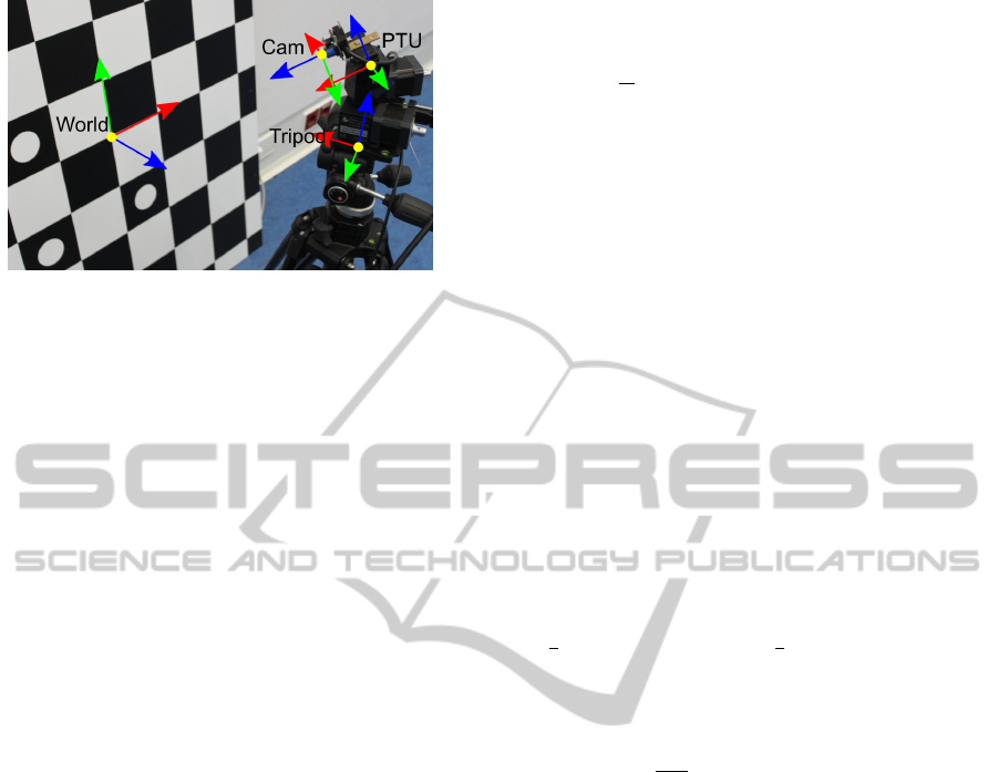
Figure 2: Setup of checkerboard calibration. The World co-
ordinate system lies at the center of the checkerboard with x
and y axes pointing along the grid and z pointing upwards.
The PTU has two coordinate systems which are rotated to-
wards each other by the current angles of the PTU. We de-
fine the coordinate system attached to the tripod as Tripod
with x pointing forward, y pointing left and z pointing up-
wards along the pan axis. The rotating system is called PTU
and actually shares the position of Tripod but is panned
and tilted. Finally, we have the camera coordinate system
Camera which is centered at the camera’s optical centre with
z pointing forward along the optical axis and x and y point-
ing right and down (thus matching pixel coordinates). Co-
ordinate systems are overlayed using colors red, green, and
blue for x, y, and z-axis.
automatize the calibration process, by providing lots
of corner measurements without having to manually
reposition the checkerboard or camera. Furthermore,
it increases the accuracy of the calibration, by having
more measurements defining the pose of the tripod
(and thereby indirectly each camera pose) relative to
the checkerboard.
Before starting the calibration, we manually ad-
justed the focal length of the camera, viewing a
Siemens star, optimizing focus at about 1 m.
3.2 Measurement Equations
From here on, we will use the notation T
A←B
to de-
scribe the transformation from coordinate system B to
A. We abbreviate the World, Tripod, PTU and Camera
systems introduced in Fig. 2 by their first letters and
append indices where required.
We have a sequence of tripod poses T
W←T
i
and for
each tripod pose we have a sequence of PTU rotations
T
T
i
←P
i j
. Furthermore, there is a transformation from
the camera coordinate system to the PTU T
P←C
(this
is assumed to be the same for all measurements). We
have a set of corner points with known world coordi-
nates x
[k]
W
which we transform to camera coordinates
via
x
[k]
C
i j
= (T
W←T
i
· T
T
i
←P
i j
· T
P←C
)
−1
x
[k]
W
. (5)
To map a point from 3D camera coordinates to
pixel coordinates, we use the OpenCV camera model
(OpenCV, 2014, “calib3d”) described by this formula
for [
u
1
u
2
] = ϕ
K
([x
1
x
2
x
3
]
>
):
[
w
1
w
2
] =
1
x
3
[
x
1
x
2
] “Pinhole model” (6a)
[
v
1
v
2
] = κ · [
w
1
w
2
] +
h
2p
1
w
1
w
2
+p
2
(r
2
+2w
1
2
)
p
1
(r
2
+2w
2
2
)+2p
2
w
1
w
2
i
(6b)
with r
2
= w
2
1
+ w
2
2
, κ = (1 + k
1
r
2
+ k
2
r
4
+ k
3
r
6
)
[
u
1
u
2
] =
f
1
v
1
f
2
v
2
+ [
c
1
c
2
] =: ϕ
K
(x), (6c)
where we join all intrinsic calibration parameters into
a vector K = [ f
1
, f
2
,c
1
,c
2
,k
1
,k
2
, p
1
, p
2
,k
3
].
The transformations T
P←C
and each T
W←T
i
are
modeled as unconstrained 3D transformations, the
PTU orientations T
T
i
←P
i j
as 3D orientations which are
initialized by and fitted to orientations
ˆ
P
i j
measured
by the PTU. The projected corner positions are fitted
to corner positions ˆz
[k]
i j
extracted from the amplitude
images.
As usual for model fitting, we solve a non-
linear least squares problem, minimizing the follow-
ing functional:
F(K,T
P←C
,[T
W←T
i
]
i
,[T
T
i
←P
i j
]
i j
) = (7)
1
2
∑
i, j,k
ˆz
[k]
i j
− ϕ
K
(x
[k]
C
i j
)
2
+
1
2
∑
i, j
T
T
i
←P
i j
−
ˆ
P
i j
2
with ϕ
K
(x
[k]
C
i j
) according to (5) and (6). We assume
that the PTU is accurate approximately to its spec-
ified resolution
2π
7000
≈ 0.05
◦
. This corresponds to
about 0.08 px and as this is about the same magni-
tude as sub-pixel corner detection, we cannot neglect
it. Therefore, the second term is scaled accordingly.
F is minimized using our general purpose least
squares solver SLoM (Hertzberg et al., 2013).
3.3 Robustified Corner Extraction
To extract corners we use the cornerSubPix method
from OpenCV. Applying the method directly to the
amplitude image turned out to be unstable if corners
are close to each other or to unrelated image gradients
(Fig. 3a). The reason is that gradients from neigh-
boring edges are wrongfully included into the refine-
ment. We have considered masking out invalid edges
from the image, but that would have required massive
rewriting of the corner detection. Instead, we project
the image to the plane where the checkerboard should
be (adding some border pixels on each side, Fig. 3b),
extract the corners in that image and back-project the
found corners to the original image (Fig. 3c). An
advantage of this procedure is that the corner ex-
tractor can always work using the same search win-
dow. By taking the back-projected corner positions as
DetailedModelingandCalibrationofaTime-of-FlightCamera
571
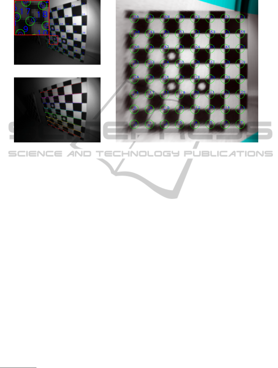
(a) Failed extraction
(c) Reprojected corners (b) Corners extracted in rectified image
Figure 3: Robustified corner extraction. Green circles show the initial guess and search window for corner refinement,
blue circles show the refined corner positions. (a) Failed corner extraction, because of unrelated gradients in the search
window. Note that for smaller search windows the extraction of the top-right corners would lose precision. (b) Using an
initial calibration and a guess of the camera pose the image is projected to the checker-board plane. We also adjust the
brightness based on the expected distance and normal vector (cf. Sec. 4.3) Areas outside the original image are continued
using the border pixels (cyan/black areas in this figure). Note that even the bottom-left corners are robustly extracted. (c) The
refined corner positions are back-projected to the original image.
measurements we automatically have their accuracies
weighted according to the amount of pixels involved
in the measurement.
This procedure requires an initial guess of the
camera intrinsics, which is taken from a previous cal-
ibration, and the pose of the camera relative to the
checkerboard, which is determined by calculating the
relative pose from a previous PTU state or by manu-
ally selecting four points in the center of the checker-
board. To ensure robustness we decided to not rely on
automatic checkerboard detection if the camera pose
is entirely unknown. Still, the only case that requires
user interaction is whenever the pose of the tripod has
been changed.
3.4 Calibration Results
We recorded 90 frames from two tripod poses by us-
ing 45 different PTU orientations each. For each
frame we recorded 8 images with 4096 µs exposure
time
2
and calculated the amplitude of the mean (com-
plex) image.
2
N.B.: Exposure times above 2000 µs require calling an
undocumented driver command
Overall, we extracted more than 4500 corners
which means that about 50 of 64 corners were visible
on average. Optimization lead to a root-mean-squares
(RMS) error of about 0.13 px. The estimated focal
length was f
1
≈ f
2
≈ 89.5 px with the camera cen-
ter at c ≈
h
79.5px
60.5px
i
. The resulting distortion pattern is
shown in Fig. 4.
The calibration was repeated with a different set
of poses and resulted in the same parameters with less
than 0.5 % discrepancy. We considered this accurate
enough for our purpose.
4 PROPOSED PIXEL MODEL
In this section we propose a physically motivated
sensor model and fit it as well as possible to the
data recorded in the previous section. It is based on
(Lange, 2000; Möller et al., 2005) and some educated
guesses on the underlying mechanisms.
As in Sec. 1.3 we follow in the description the path
of light from the LED through the scene to the sensor.
We assume that the measurement of each single pixel
is solely caused by the reflection of a surface patch
ICINCO2014-11thInternationalConferenceonInformaticsinControl,AutomationandRobotics
572

Figure 4: Lens Distortion. The arrows point from the the-
oretical undistorted point to the distorted point. Distortions
below 1 px are not shown. The image border is marked
black. As common for wide-angle lenses the distortion near
the borders is very high.
Figure 5: Path of the light from the LED, reflected by a
white wall to the camera. The position of the LED relative
to the camera is d
LED
, and x
•
denotes the coordinates of the
wall patch in each coordinate system. The normal vector of
the surface is called n.
with normal n and a position x
Cam
relative to the cam-
era center. We also assume that the surface patch is a
perfect Lambertian reflector with albedo α. Knowing
the position of the LED relative to the camera d
LED
,
we determine the position of the surface patch relative
to the LED x
LED
:= x
Cam
− d
LED
. This is visualized
in Fig. 5.
4.1 Emitted Light Wave
First of all, the emitted light wave is not a sinusoidal.
By design, it is closer to a rectangular wave, but
due to hardware restrictions it is smoothed near the
switchover points and not necessarily constant else-
where. All we assume is that the emitted light can be
described by a continuous function ψ(t) with a peri-
odicity
1
ν
.
For simplicity we can assume that ν =
1
4
(by ar-
bitrarily choosing the unit of ν) and therefore ψ(t) =
ψ(t + 4). We will also not model ψ directly but its
integral Ψ over half the phase. By subtracting half
the integral over the entire phase, Ψ becomes anti-
periodic with Ψ(t) = −Ψ(t +2):
Ψ(t) :=
Z
t+2
t
ψ(τ)dτ −
1
2
Z
4
0
ψ(τ)dτ
| {z }
=:Ψ
0
. (8)
Because the scale and time offset of ψ and thus Ψ
are arbitrary, we choose them so that Ψ(0) = 0 and
Ψ(1) = 1. We will then model Ψ using two polyno-
mials Ψ
s
and Ψ
c
of order 8 with:
Ψ(t) =
Ψ
s
(t)
|
t
|
≤
1
2
Ψ
c
(t − 1)
|
t − 1
|
≤
1
2
−Ψ(t −2) t >
3
2
−Ψ(t +2) t < −
1
2
,
(9)
where the transitions between Ψ
s
and Ψ
c
are modeled
to be twice continuously differentiable. The resulting
Ψ is later shown in Fig. 7.
4.2 Vignetting
The lens in front of the LED does not distribute the
light uniformly which causes strong vignetting. We
model this effect depending on the direction of the
light exiting the LED by a bi-polynomial ` depending
on
1
x
LED
3
h
x
LED
1
x
LED
2
i
, with
`([
u
1
u
2
]) =
3
∑
i=0
i
∑
j=0
l
j,i− j
u
j
1
u
i− j
2
. (10)
We write `(x) := `(
1
x
3
[
x
1
x
2
]) and collect the coefficients
into an upper-left matrix L = (l
i j
)
i+ j≤3
, where we nor-
malize l
00
:= 1.
4.3 Scene Interaction
If we assume perfect Lambertian reflection, the
amount of reflected light is proportional to the albedo
α
i,p
and the scalar product of the direction of incom-
ing light x
LED
i,p
/
x
LED
i,p
with the surface normal n
i
(whenever a value depends on a camera pose T
i
or a
pixel p, we will from now denote this by indexes
i,p
).
Also, it is reciprocally proportional to the squared dis-
tance from the LED.
We combine this with the vignetting from the pre-
vious section and the integration time t
I
to calculate
the expected effective amplitude
A
[t
I
]
i,p
= t
I
· α
i,p
· `(x
LED
i,p
)
h
x
LED
i,p
,n
i
i
x
LED
i,p
3
. (11)
Note that α
i,p
will contain the normalization factors
of the emitted light (Ψ(1) = 1) and the vignetting
(`(0) = 1).
The phase offset is calculated by dividing the dis-
tance travelled
x
LED
i,p
+
x
Cam
i,p
by the speed of light.
As the speed of light equals the product of wavelength
λ and frequency ν, and we chose ν =
1
4
(cf. Sec. 4.1)
this can be simplified to
∆t
i,p
= 4 ·
k
x
LED
i,p
k
+
x
Cam
i,p
λ
. (12)
DetailedModelingandCalibrationofaTime-of-FlightCamera
573

4.4 Photon Response Curve
The actual pixel measurements are not linear in the
received light. As in (Lange, 2000) we assume that
each pixel consists of two “bins” A and B. We as-
sume that each bin has a response-curve g
A
, g
B
and
the pixel measurement is the difference between those
bins offset by γ. Bin A is assumed to accumulate for
0 ≤ t < 2 and B for 2 ≤ t < 4
s
[k]
i,p
= γ
p
+ g
A
p
Z
k+2
k
z
i,p
(t)
dt − g
B
p
Z
k+4
k+2
z
i,p
(t)
dt
= γ
p
+ g
A
p
A
[t
I
]
i,p
(Ψ
0
+ Ψ(∆t
i,p
+ k))
− g
B
p
A
[t
I
]
i,p
(Ψ
0
− Ψ(∆t
i,p
+ k))
.
(13)
By design, g
A
and g
B
are almost identical and as their
values cannot be measured individually we make a
simplification by subtracting s
[k]
i,p
−s
[k+2]
i,p
. This cancels
out the γ
p
and g
A
p
and g
B
p
can be joined to a single
function g
S
p
(x) := g
A
p
(x) + g
B
p
(x):
s
[k]
i,p
− s
[k+2]
i,p
= g
S
p
A
[t
I
]
i,p
(Ψ
0
+ Ψ(∆t
i,p
+ k))
− g
S
p
A
[t
I
]
i,p
(Ψ
0
− Ψ(∆t
i,p
+ k))
.
(14)
We model g
S
p
using a rational polynomial
g
S
p
(x) = x
x + g
0
x + g
1
, (15)
where we assume that the coefficients between pixels
are similar enough to be modeled by the same coef-
ficients G = [g
0
,g
1
]. Finally, we capture (14) into a
helper function:
g
D
(A,Ψ
0
,Ψ) = g
S
(A(Ψ
0
+ Ψ)) − g
S
(A(Ψ
0
− Ψ))
= 2AΨ ·
1 +
g
1
(g
0
−g
1
)
A
2
Ψ
2
−(AΨ
0
+g
1
)
2
. (16)
4.5 Fixed Pattern Noise (FPN)
Due to different internal signal propagation times, in-
dividual pixels have a time-offset δt
p
, which must be
added to the time offsets ∆t
i,p
before being inserted
into (14). Furthermore, pixels have a slightly differ-
ent gain, which we model by multiplying each g
p
by
a factor h
p
≈ 1.
4.6 Complete Pixel Model
Summarizing the previous subsections, we model
each complex-valued pixel at p, with
I
[t
I
]
i,p
=
s
[0]
i,p
− s
[2]
i,p
,s
[1]
i,p
− s
[3]
i,p
(17)
= h
p
·
g
D
(A
[t
I
]
i,p
,Ψ
0
,Ψ(∆t
i,p
+ δt
p
)),
g
D
(A
[t
I
]
i,p
,Ψ
0
,Ψ(∆t
i,p
+ δt
p
+ 1))
.
(18)
(a) Setup, Coordinate systems
(b) Corners
(c) White mask
Figure 6: White wall with markers. We covered the floor
with low-reflective textile to limit multi-path reflections.
Overall, the sensor model depends on the coefficients
of the emitted light wave Ψ
[k]
c
, Ψ
[k]
s
and Ψ
0
which we
collect into a vector Ψ
p
, the parameters L of the vi-
gnetting polynomial, the coefficients G of the photon
response curve, and the FPN images H = (h
p
)
p
and
δT = (δt
p
)
p
.
5 PIXEL CALIBRATION
In this section we describe how we calibrate the previ-
ously proposed model. We also show how our model
can be used to obtain high dynamic range (HDR) im-
ages and propose a way to invert our model, i.e., to
actually compute distance values using the measure-
ments of the sensor.
5.1 White Wall Recordings
For calibration of each sensor pixel we need many
measurements of equal albedo α
i,p
= α and with a
known position and surface normal relative to the
camera and the LED. We chose to record an ordinary
white-painted wall, to which we attached markers as
illustrated in Fig. 6a.
We measured the distances between the markers
using a tape measure. We defined the wall coordinate
system to originate from the first marker, with the sec-
ond marker in x-direction and both others on the x-y-
plane. Having four markers and six distances between
them, we have an overdetermined system. Also, view-
ing the four markers in a camera image is sufficient to
determine the pose of the camera relative to the wall.
As in Sec. 3, we recorded the wall using the same
tripod position for various PTU orientations. This
again increases the number of constraints defining
the tripod pose relative to the plane and also semi-
automatizes the process of obtaining calibration val-
ICINCO2014-11thInternationalConferenceonInformaticsinControl,AutomationandRobotics
574

ues. For each PTU orientations we made recordings
with various integration times, starting from 16 µs up
to 4096µs.
The camera poses where optimized using the same
functional (7) as in Sec. 3, but this time fixing the
camera intrinsics K and the transformation from cam-
era to PTU coordinates T
P←C
. The resulting camera
poses will be considered as groundtruth from now on
and we will simply call them T
i
, ignoring the state and
index of the PTU.
From the already known camera intrinsics K we
can calculate a direction vector v
p
for each pixel p.
Using the camera pose T
i
we can calculate the vector
x
Cam
i,p
going from the camera center to the center of the
corresponding patch at the wall.
Knowing also the displacement d
LED
of the LED
relative to the camera
3
, allows us to calculate x
LED
i,p
=
x
Cam
i,p
− d
LED
(cf. Fig. 5).
The camera pose and intrinsics are also used to
project the positions of the markers into the image in
order to exclude these pixels from the calibration by
providing a mask M
i
of pixels assumed to be white
(cf. Fig. 6c).
5.2 Optimization
For now, we assume that all pixel measurements are
independent, i.e., we neglect influence of lens scatter-
ing and multi-path reflections.
We use the ground truth values from the previ-
ous subsection and the measured images for different
poses T
i
and different integration times t
I
, viewed as
complex images
ˆ
I
i,t
I
= ( ˆs
[0]
i,t
I
− ˆs
[2]
i,t
I
, ˆs
[1]
i,t
I
− ˆs
[3]
i,t
I
), (19)
to assemble a functional
F(Ψ
p
,G,L,H,δT ) =
∑
i,t
I
,p
I(p) −
ˆ
I
i,t
I
(p)
2
(20)
We alternately optimize Ψ
p
, G and L using (Hertzberg
et al., 2013) and the FPN parameters H, δT using a
linearized least squares procedure per pixel.
5.3 Inverse Model
To invert the model we need to solve (18) for the un-
known amplitude A
[t
I
]
i,p
and phase-shift ∆t
i,p
. Since
these calculations are independent for all pixels and
poses, we abbreviate A = A
[t
I
]
i,p
and
d
0
= ˆs
[0]
i,t
I
− ˆs
[2]
i,t
I
d
1
= ˆs
[1]
i,t
I
− ˆs
[3]
i,t
I
, (21)
Φ
0
= AΨ(∆t
i,p
) Φ
1
= AΨ(∆t
i,p
+ 1). (22)
3
This is only measured manually at the moment but
small inaccuracies have negligible influence here.
Figure 7: Integrated light wave Ψ modeled as pseudo sine
Ψ
s
(red) and pseudo cosine Ψ
c
(green). Ψ is anti-periodic
with Ψ(t) = −Ψ(t + 2). Ψ
s
and Ψ
c
are modeled as poly-
nomials with C
2
-transitions at k +
1
2
, for k ∈ Z. The blue
graph is the ratio of sine over cosine, and the black graph
is the pseudo-atan calculated from the ratio and shifted ac-
cording to the signs of Ψ. The turquoise line is the deviation
of the pseudo-atan from the actual inverse, scaled by 100.
At first we ignore the fixed-pattern offset δt
i,p
and
only solve for Φ
0
, and Φ
1
, using the fact that
|
Φ
0
|
+
|
Φ
1
|
≈ A. This is done using a fixpoint iteration based
on (16) starting with
Φ
0
= d
0
Φ
1
= d
1
. (23)
The next step is to compute ∆t
p
from Φ
0
and Φ
1
.
For that we need the pseudo-atan corresponding to
the pseudo-sine Ψ
s
and pseudo-cosine Ψ
c
. This is ob-
tained during the calibration by once fitting an 8
th
or-
der polynomial Ψ
a
to Ψ
a
(Ψ
s
(t)/Ψ
c
(t)) ≈ t and then
use it here in the inverse model.
5.4 High-Dynamic-Range
Capturing multiple recordings with different integra-
tion times of a static scene we can use our model to
produce high dynamic range (HDR) images. This is
done using a similar fixpoint iteration as in the pre-
vious subsection. Indeed the previous method can be
seen as a special case, where only a single image is
provided.
5.5 Results
In Fig. 7 we show the graph of the calibrated pseudo-
sine, -cosine and -atan function. We see that the func-
tion is closer to a triangular wave than to a sine wave,
indicating that the original signal is close to a rectan-
gular wave.
6 LENS SCATTERING
The lens that comes with the Camboard Nano can be
considered as rather low-cost and has significant lens
scattering and lens flare effects. What happens is that
DetailedModelingandCalibrationofaTime-of-FlightCamera
575

light entering the lens is reflected inside the lens cas-
ing and captured by neighboring pixels or entirely dif-
ferent pixel. For ToF cameras this not only results in
slight amplitude changes, but more importantly in dis-
tortions of the measured phases (and thus distances)
towards brighter light sources, because pixel phases
are a mixture of the actual phase and a halo created
by a strong light source with a phase corresponding
to the distance of the light source.
6.1 Measuring Scattering Effects
To measure the lens scattering, we set up an area
of highly non-reflective textile and placed a retro-
reflecting disc inside it. Then we made multiple high-
dynamic-range recordings of this area once with the
retro-reflecting disc and once without it. We calcu-
lated the complex valued difference image – which
under ideal circumstances would only show the disc.
Fig. 8a shows an example.
In these difference images D
i
we declared every
pixel u ∈ Ω above a threshold Θ as being part of the
blob B
i
causing the scattering. Images with too few
blob pixels are ignored.
B
i
(u) =
(
D
i
(u) D
i
(u) > Θ
0 else.
(24)
Everything outside this blob and a safety radius of
2px is assumed to be caused by lens scattering. For
that we define a mask set M
i
:
M
i
=
u ∈ Ω; ∀
v,
k
v−u
k
<2
: D
i
(v) ≤ Θ
. (25)
6.2 Scattering Model
In this paper we restrict to point symmetrical and
translation invariant scattering, leaving out non-
symmetries and lens flare effects.
This can be modeled as convolution with a point
spread function (PSF) Q for which
D
i
= B
i
∗ Q, (26)
where ∗ expresses a convolution operation with zero
border condition:
(B ∗ Q)(u) =
Z
v∈Ω
B(v) · Q(u − v)dv. (27)
For brevity, we define a (semi) scalar product and cor-
responding semi-norm
4
over M
i
as
h
f ,g
i
M
i
=
∑
u∈M
i
f (u)g(u), (28)
k
f
k
M
i
=
q
h
f , f
i
M
i
. (29)
4
Because we are masking out pixels, we can have non-
zero images with zero norm.
We then try to find a PSF Q which minimizes
F(Q) =
1
2
∑
j
k
D
i
− (B
i
∗ Q)
k
2
M
i
, (30)
where we model Q as a sum of Gaussian-shaped func-
tions Q
j
with a fixed set of σ
j
Q(u) =
∑
j
q
j
Q
j
(u) =
∑
j
q
j
exp
−
|
u
|
2
2σ
2
j
. (31)
Inserting (31) into (30) and exploiting the linearity of
convolutions and the bilinearity of the scalar product,
we calculate
F(Q) =
1
2
∑
i
k
D
i
k
2
M
i
− 2
h
D
i
,B
i
∗ Q
i
M
i
+
k
B
i
∗ Q
k
2
M
i
(32)
=
1
2
∑
i
k
D
i
k
2
M
i
| {z }
=:c
−
∑
j
∑
i
B
i
∗ Q
j
,D
i
M
i
| {z }
=:b
j
q
j
+
1
2
∑
j,k
∑
i
B
i
∗ Q
j
,B
i
∗ Q
k
M
i
| {z }
=:A
jk
q
j
q
k
. (33)
Collecting the coefficients q
j
into a vector q this leads
to a simple linear least squares problem:
F(Q) = min
Q
! ⇔
1
2
q
>
Aq − b
>
q +
1
2
c = min
q
! (34)
⇔ Aq = b. (35)
6.3 Inverse Lens Scattering
The previous subsections described how we estimated
the point spread function, describing the scattering.
We will now show how this is compensated using
Fourier transformations. The measured image
˜
I can
be computed from the un-scattered image as
˜
I = I +
(I ∗ Q). Using the identity δ ∗ I = I and applying the
convolution theorem, we can write
˜
I = (δ + Q) ∗ I = F
−1
F (δ + Q) · F (I)
(36)
⇔ I = F
−1
F (
˜
I)/F (δ + Q)
. (37)
As F δ ≡ 1 and Q is small, we can safely divide by
F (δ + Q) in the Fourier space. Also, as Q is fixed,
we only need to compute 1/(F (δ + Q)) once and
can then compensate arbitrary images by only calcu-
lating one forward Fourier transform, a per-element
multiplication of the Fourier images and one back-
ward Fourier transform. This can be done directly
using complex images, since we always have two cor-
responding values per pixel.
6.4 Results
Fig. 8 summarizes the effect of compensating scatter-
ing effects on different kind of images. The resulting
point spread function is shown in Fig. 9.
ICINCO2014-11thInternationalConferenceonInformaticsinControl,AutomationandRobotics
576
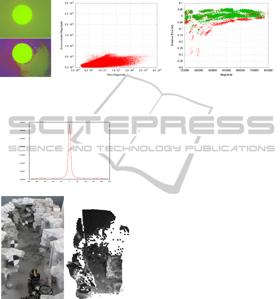
(a) Original and Decon-
voluted test image
(b) Magnitude of error in test images before and
after deconvolution
(c) Distance difference to ground-truth before
(red) and after (green) deconvolution
Figure 8: Figures (a) and (b) show the results of deconvoluting the training images. Figure (c) shows the difference to
a checkerboard ground-truth distance, before and after compensating the scattering effect dependent on the magnitude of
received light.
Figure 9: Point spread function Q as a function of the radius.
(a) Mockup with markers (b) 3D view
Figure 10: Mockup with markers.
7 RESULTS
To verify our combined calibration efforts, we set up
a Styrofoam mock-up (Fig. 10), motivated by an ur-
ban search and rescue scenario. We marked several
spots inside the mock-up and measured the distance
to the camera using a tape measure which we used as
ground-truth for comparison.
We then made 64 recordings of the scene with dif-
ferent integration times from 8 to 8192µs and we cal-
culated the mean difference and standard deviation for
several evaluation methods. The results are shown in
Fig. 11
8 CONCLUSIONS AND FUTURE
WORK
The main contribution of this paper is to provide a
ToF sensor model which handles different integration
times and thus is capable of producing HDR images.
In contrast to previous calibration approaches we try
to generate an accurate model from the beginning in-
stead of adjusting the simplistic model given in (4).
Being capable of recording HDR images we showed a
straight-forward method to calibrate and compensate
lens-scattering effects. We believe that exact HDR
images are also required to reliably compensate ef-
fects of multi-path-reflections.
Furthermore, no extensive calibration equipment
is required. In principle, a checkerboard and a white
wall with self-printed markers is sufficient. However,
some kind of automatically moving device (such as a
PTU or a robot arm) helps to significantly reduce the
manual work and increase the accuracy. We conclude
by listing some phenomena left out in this paper, we
esteem worthwhile investigating.
8.1 Temperature Compensation
It should be possible to take the temperature of the
sensor and LED into account in the sensor model. As
DetailedModelingandCalibrationofaTime-of-FlightCamera
577
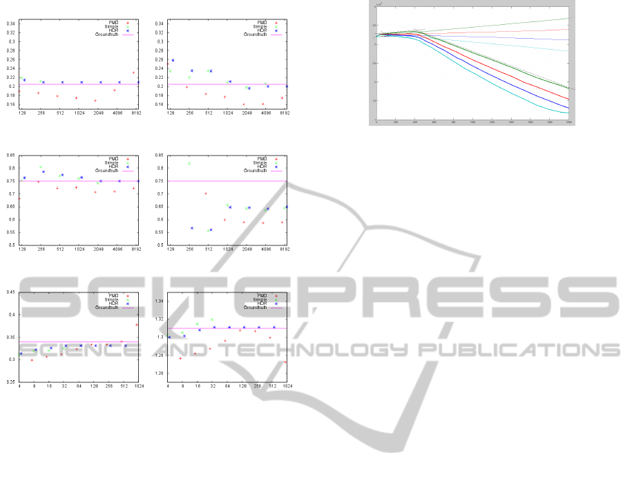
(a) White 205mm (b) Black 205mm
(c) White 750mm (d) Black 750mm
(e) Reflector 340mm (f) Reflector 1310mm
Figure 11: Distance measurements of pixels with hand-
measured groundtruth. Green crosses are our inverse model
applied to single measurements, blue stars are HDR record-
ings accumulated starting from 4 µs. Red pluses mark the
values obtained from the manufacturer’s driver and the vio-
let bar is the hand-measured groundtruth for comparison.
On close ranges (a) or on highly reflective targets (e, f) sin-
gle measurements quickly saturate, while the HDR model
still works, ignoring saturated values. The manufacturer
seems to model saturated values better, however the ben-
efit of HDR recordings is apparent. The black are of the
marker in (d) is overlayed by lens-scattering and multi path
reflections.
both temperatures are measured with an unknown de-
lay, this also requires modeling how the actual sen-
sor temperature changes given certain integration or
waiting times and ambient temperature (which also
usually is not known exactly). Furthermore, the tem-
perature may have different effects on the generated
light wave and the photon response curve. This is hard
to determine since the temperature of both cannot be
varied independently.
8.2 Ambient Light Effects
Fig. 12 shows how strong ambient light can have non-
trivial effects on the generated signal. Partially, this is
compensated by SBI (Möller et al., 2005, §4.2), but
this compensation is not perfect. We left this calibra-
Figure 12: Raw values of PMD sensor, showing non-
linearities and saturation effects. Each line are raw values
of a single pixel in each sub-image. The right axis is the
integration time in µs. Thick lines are with high back-light
illumination, thin lines with almost no back-light. Notice
that none of the thick curves is monotonic and all have sub-
stantial bends at approximately the same integration time.
This behavior is different for different pixels and also de-
pends on the temperature of the sensor.
tion out, since pure ambient light is not directly mea-
surable by our sensor and has very different effects on
different pixels. Also our application will usually as-
sume very little ambient light, which we assume to be
negligible.
8.3 Multi-Path Reflections
Very complex problems arise if multi-path reflexions
are to be considered. We think, essentially this can
only be solved by applying an actual ray-caster to a
model of the scene and successively refine this model
(Jimenez et al., 2012). The problem gets arbitrary
complex, if surfaces with non-Lambertian reflection
(such as mirrors or retro-reflectors) or surfaces out-
side the camera’s field of view have to be considered.
ACKNOWLEDGEMENTS
This work has partly been supported under DFG grant
SFB/TR 8 “Spatial Cognition”.
REFERENCES
Castaneda, V., Mateus, D., and Navab, N. (2011). SLAM
combining ToF and high-resolution cameras. In Ap-
plications of Computer Vision (WACV), 2011 IEEE
Workshop on, pages 672–678.
Fuchs, S. and Hirzinger, G. (2008). Extrinsic and depth
calibration of ToF-cameras. In Computer Vision and
Pattern Recognition, 2008. CVPR 2008. IEEE Confer-
ence on, pages 1–6.
Fuchs, S. and May, S. (2008). Calibration and registra-
tion for precise surface reconstruction with time-of-
flight cameras. Int. J. Intell. Syst. Technol. Appl.,
5(3/4):274–284.
ICINCO2014-11thInternationalConferenceonInformaticsinControl,AutomationandRobotics
578

Hertzberg, C., Wagner, R., Frese, U., and Schröder, L.
(2013). Integrating generic sensor fusion algorithms
with sound state representation through encapsulation
of manifolds. Information Fusion, 14(1):57–77.
Jimenez, D., Pizarro, D., Mazo, M., and Palazuelos, S.
(2012). Modelling and correction of multipath inter-
ference in time of flight cameras. In Computer Vision
and Pattern Recognition (CVPR), 2012 IEEE Confer-
ence on, pages 893–900.
Kahlmann, T., Remendino, F., and Ingensand, H. (2006).
Calibration for increased accuracy of the range imag-
ing camera SwissRanger. In TM Proceedings of the
ISPRS Com. V Symposium.
Lange, R. (2000). 3D Time-of-Flight Distance Mea-
surement with Custom Solid-State Image Sensors in
CMOS/CCD-Technology. PhD thesis, University of
Siegen.
Lindner, M. and Kolb, A. (2006). Lateral and depth cali-
bration of PMD-distance sensors. In Bebis, G., Boyle,
R., Parvin, B., Koracin, D., Remagnino, P., Nefian,
A., Meenakshisundaram, G., Pascucci, V., Zara, J.,
Molineros, J., Theisel, H., and Malzbender, T., edi-
tors, Advances in Visual Computing, volume 4292 of
Lecture Notes in Computer Science, pages 524–533.
Springer Berlin Heidelberg.
May, S., Fuchs, S., Droeschel, D., Holz, D., and Nüchter, A.
(2009). Robust 3D-mapping with time-of-flight cam-
eras. In Proceedings of the 2009 IEEE/RSJ Interna-
tional Conference on Intelligent Robots and Systems,
IROS’09, pages 1673–1678, Piscataway, NJ, USA.
IEEE Press.
Möller, T., Kraft, H., Frey, J., Albrecht, M., and Lange, R.
(2005). Robust 3d measurement with pmd sensors. In
In: Proceedings of the 1st Range Imaging Research
Day at ETH, pages 3–906467.
Mure-Dubois, J. and Hügli, H. (2007). Optimized scattering
compensation for time-of-flight camera. Proc. SPIE,
6762:67620H–67620H–10.
Newcombe, R. A., Izadi, S., Hilliges, O., Molyneaux, D.,
Kim, D., Davison, A. J., Kohli, P., Shotton, J., Hodges,
S., and Fitzgibbon, A. W. (2011). KinectFusion: Real-
time dense surface mapping and tracking. In ISMAR,
pages 127–136.
OpenCV (2014). OpenCV. http://opencv.org.
PMDtechnologies (2012). pmd[vision] CamBoard nano.
http://www.pmdtec.com/products_services/
reference_design.php. last checked 2014-01-10.
Sabov, A. and Krüger, J. (2010). Identification and correc-
tion of flying pixels in range camera data. In Pro-
ceedings of the 24th Spring Conference on Computer
Graphics, SCCG ’08, pages 135–142, New York, NY,
USA. ACM.
Weingarten, J., Gruener, G., and Siegwart, R. (2004). A
state-of-the-art 3D sensor for robot navigation. In In-
telligent Robots and Systems, 2004. (IROS 2004). Pro-
ceedings. 2004 IEEE/RSJ International Conference
on, volume 3, pages 2155–2160 vol.3.
DetailedModelingandCalibrationofaTime-of-FlightCamera
579
