
Fuzzy Rule Bases Automated Design with Self-configuring
Evolutionary Algorithm
Eugene Semenkin and Vladimir Stanovov
Department of System Analysis and Operations Research, Siberian State Aerospace University,
“Krasnoyarskiy Rabochiy” avenue, 31, krasnoyarsk, 660014, Russia
Keywords: Genetic Fuzzy Systems, Fuzzy Rule Base Classifiers, Automated Design, Evolutionary Algorithms.
Abstract: Self-configuring evolutionary algorithm of fuzzy rule bases automated deign for solving classification
problems, which combines Pittsburgh and Michigan approaches, is introduced. The evolutionary algorithm
is based on the Pittsburgh approach where every individual is a rule base and the Michigan approach is used
as a mutation operator. A self-configuration method is used to adjust probabilities of the usage of selection,
mutation and Michigan part operators. Testing the algorithm on a number of real-world problems
demonstrates its efficiency comparing to several other commonly used approaches.
1 INTRODUCTION
Today the most popular methods for the automated
design of fuzzy rule bases and fuzzy systems are
evolutionary algorithms. Genetic algorithms (GA)
are mostly used, as well as their modifications, so
this field received the name of genetic fuzzy systems
(Cordon et al., 2001). The techniques for forming
fuzzy controllers take a special place here, but in this
paper we will focus on classification problems
solving.
The first works on data classification with fuzzy
rule bases appeared in the 90’s (Wang et al., 1992),
and several methods were developed, for example
(Alcala et. al., 2007) and (Fernández et. al, 2009). In
most of the works the design of a fuzzy logic system
was transformed into the problem of choosing rules
from a predefined set of good individual rules. There
are basically two approaches – the Michigan
approach (building rules) and the Pittsburg approach
(building an entire rule base). The first method
allows the formation of individual rules which
describe some part of the sample, but without a rule
base, so that classification is impossible. The second
method forms an entire rule base and is much more
difficult in terms of computational efforts, but it
provides a ready solution to the problem. Today
there appear more and more methods that combine
these two approaches (Bodenhofer et. al., 1997).
In this paper we consider a modification of an
algorithm, combining the Pittsburg and Michigan
approaches, that was described in (Ishibuchi et al.,
2005). One of the disadvantages of this algorithm, as
well as of any other evolutionary method, is the
existence of several genetic operators that influence
the properties of the search algorithm and must be
properly adjusted according to each problem. So, it
seems reasonable to use some self-configuration
methods, which adjust the operators’ application
probabilities during the algorithm run.
2 CLASSIFICATION WITH
FUZZY RULE BASES
Let the classification problem be given in n-
dimensional space with m measurements and M
classes. Every measurement is represented as a
vector x
p
=(x
p1
, x
p2
… x
pn
), p=1…m. We assume that
every variable has been normalized into the [0,1]
interval. The rules used look as follows:
R
q
: if X
1
is A
q,1
and X
2
is A
q,2
and … and X
n
is
A
q,n
then
X is from class C
q
with level CF
q
.
R
q
is a rule, A
q,i
is a fuzzy set, C
q
is the number of
the corresponding class, CF
q
is the rule weight. This
is the standard rule representation, which is used in
classification problems. Unlike some other
representations, this rule has a weight CF
q
, which is
determined using the learning sample.
318
Semenkin E. and Stanovov V..
Fuzzy Rule Bases Automated Design with Self-configuring Evolutionary Algorithm.
DOI: 10.5220/0005062003180323
In Proceedings of the 11th International Conference on Informatics in Control, Automation and Robotics (ICINCO-2014), pages 318-323
ISBN: 978-989-758-039-0
Copyright
c
2014 SCITEPRESS (Science and Technology Publications, Lda.)

There are four different variables’ space partitions
into 2, 3, 4 and 5 fuzzy sets plus a “don’t care” term,
so that a coded rule is an integer string with a
number from 0 to 14.
Figure 1: Fuzzy sets partitions.
The class number C
q
and the weight value CF
q
are captured separately. The “don’t care” term
means that the value of this variable is not
considered in the rule. This kind of technique allows
the creation of more general rules, reduces their
number and length, and gradually simplifies the rule
base. The compatibility grade of a certain
measurement x
p
in the rule R
m
is calculated as the
product of compatibility grades over all the
variables. For the ignored variables the compatibility
grade is considered as equal to one. Alternatively, a
minimum operator can be used instead of
multiplication.
The class number and the weight value are
calculated based on the confidence value in the same
way as in (Ishibuchi et al., 2005). For the rule R
m
the
class C
q
, is set if the confidence value for this class
is maximal among all other classes. If the confidence
value is less than 0.5, the rule is not generated. The
classification procedure is performed using the
winner-rule principle. This means that the rule that
has the highest product of compatibility by the
weight value is the winner rule. The measurement is
classified into the class number equal to the winner
rule class.
3 HYBRID EVOLUTIONARY
ALGORITHM OF FUZZY RULE
BASES FORMATION
The developed algorithm implements the Ishibuchi
approach (Ishibuchi et al., 2005). This algorithm can
be described in the following way:
Population initialization;
Rule bases fitness calculation;
Selection, crossover, mutation;
Applying the Michigan part to every individual;
Forming a new generation;
If the stop condition is satisfied, then exit, else
go to step 2;
The Michigan part contains the following steps:
Classify the learning sample with a rule base and
set the rules’ fitness;
Generate or delete rules from the population with
one of the methods;
Return the obtained rules base into the Pittsburg
part.
The number of rules in the algorithm is not fixed
and it can be changed for every individual.
Nevertheless, the maximum number of rules is set.
So, the rule base is a matrix where every row is the
rule. Some of these rules can be muted and have
zero weight. During the initialization step every rule
of the rule base is formed based on randomly
selected examples from the learning sample. To
form a rule, the compatibility grades are calculated
for every term, and the greater these numbers are,
the more chances this fuzzy set has of being
included in the rule.
The fitness is calculated as a combination of
three objectives: the error in the learning sample in
percent, the number of rules in the base and the
overall length of all the rules. For the first criterion
the weight is equal to 100, and for the two others –
1. Multi-objective approaches can also be used, and
there are several examples, such as (Fazzolari et al.,
2013).
In a genetic algorithm, three selection types are
used – fitness proportional, rank-based and
tournament selection with a tournament size of
three. The crossover operator combines the genetic
information of parents and generates a new rule base
using the parents’ rules. The number of rules for the
offspring is equal to a random number from 1 to the
overall number of parents’ rules, if it does not
exceed the stated maximum number of rules.
The mutation operator is almost the same as the
mutation in standard GA, i.e. the mutation
probability depends on the number of rules and for
an average mutation equal to 1/(n*|S|), |S| is the
number of rules in the rule base. The weak and
strong mutations have probabilities 1/(3*n*|S|) and
3/(n*|S|) respectively in this algorithm.
The Michigan stage contains two main
operations – adding new rules and deleting them.
There are three possible types of Michigan stage –
only adding new rules, only deleting rules, and
replacement of rules by deleting and adding new
rules instead. The adding of new rules involves two
methods – genetic and heuristic. The heuristic
method includes new rules into the base, which are
formed using the misclassified measurements from
the sample in the same way as during the
initialization procedure. In the genetic method the
FuzzyRuleBasesAutomatedDesignwithSelf-configuringEvolutionaryAlgorithm
319

number of objects classified by this rule is used as a
fitness value. The rules are selected, then they
undergo crossover and mutation to form an
offspring. The tournament selection, uniform
crossover and average mutation are used. The
genetic and heuristic approaches are applied with
probability of 0,5. During the deleting procedure the
rules with the lowest fitness are removed from the
base.
The number k of deleted or added rules depends
on the current number of rules in the base and is
calculated so that 5(k-1) < |S| <= 5k. If the number
of rules in the base reaches the given maximum
number, new rules are not added to it.
The forming of a new population in the Pittsburg
part includes the best offspring and parents into the
new generation.
4 EVOLUTIONARY
ALGORITHM
SELF-CONFIGURATION
TECHNIQUE
Self-configuration means setting the application
probabilities of evolutionary operators based on the
success of the operators. Self-configuration needs to
be used as the algorithm efficiency highly depends
on the operators used.
The applied self-configuration method
(Semenkin et al., 2012-1) is based on encouraging
those operators which received the highest total
fitness in the current generation. This approach has
proved its efficiency in the solving of hard real
world optimization problems (Semenkin et al., 2012-
2, Semenkin et al., 2014) and has been
recommended for practical use.
Let z be the number of different operators of i-th
type. The starting probability values are set to
p
i
=1/z. The success estimation for every type of
operator is performed based on the averaged fitness
values:
1
1
, 1, 2,...,
1
i
i
n
ij
j
i
n
j
f
A
vgFit i z
where n
i
is the number of offspring formed with i-th
operator, f
ij
is the fitness value of j-th offspring,
obtained with i-th operator, AvgFit
i
is the average
fitness of the solutions, obtained with i-th operator.
Then the probability of applying the operator,
whose AvgFit
i
value is the highest among all the
operators of this type, is increased by (zK-K)/(zN),
and the probabilities of applying other operators are
decreased by K/(zN), where N is the number of
evolutionary algorithm generations, K is the constant
equal to 0,5.
The probabilities of the selection operators, the
mutation operators and the Michigan operators are
adjusted during the algorithm operation. In the first
generation equal probabilities are applied to all the
operators. For example, for the Michigan operators,
the probabilities of adding, deleting and replacement
procedures are equal when the algorithm starts.
5 ALGORITHM
IMPLEMENTATION AND
TESTING RESULTS
One of the advantages of this algorithm is that for
every rule in the base the compatibility grades for
every variable, as well as the class number and
weight, can be calculated only once and then
updated only for those rules that changed during the
algorithm run. This allows the sample to be used
fewer times, that results in a better computation
time.
Six heterogeneous classification problems from
the UCI repository (Asuncion et al., 2007) and the
KEEL repository (Alcalá-Fdez et al., 2009) were
chosen for the approach performance evaluation,
namely:
Australian credit card problem, 690 instances, 14
variables, 2 classes – Australian;
German bank client classification problem, 1000
instances, 24 variables, 2 classes – German;
Image segments classification problem, 2310
instances, 19 variables, 7 classes – Segment;
Text recognition sections classification problem,
5472 instances, 10 variables, 5 classes –
Pageblocks;
Nasal and oral sounds classification problem,
5404 instances, 5 variables, 2 classes, –
Phoneme;
Satellite image pixels classification problem,
6435 instances, 36 variables, 6 classes, –
Satimage.
To measure the classification quality the 10-fold
cross-validation procedure was used. In this method
the sample is split into 10 parts, 9 of them are used
as a learning sample, and the residual part as a test
sample, and then the parts are exchanged with each
other. The procedure is performed 10 times, so that
ICINCO2014-11thInternationalConferenceonInformaticsinControl,AutomationandRobotics
320

all the instances have been in the test sample at least
once. All the cross-validation procedures were
repeated three times, and the accuracy values on the
test and learning samples were averaged.
The maximum number of rules was set to 40 for
all the problems, the number of individuals in the
population – 100, the number of generations – 500,
the minimum probability of operators’ application
for self-adjustment – 0,125. Neural network models
and SVMs were built for all the problems using the
STATISTICA 10 program.
To see the effect of self-adjustment on the
algorithm performance, a set of tests of the standard
algorithm were performed with the parameters
presented in table 1.
Table 1: Algorithm configurations.
Configuration Selection type Mutation type
1
Proportional
Weak
2 Average
3 Strong
4
Rank
Weak
5 Average
6 Strong
7
Tournament (2)
Weak
8 Average
9 Strong
The next table represents a comparison of the
self-configured and standard algorithm efficiency for
six problems. The average classification rate of the
standard algorithm is also included.
Table 2: Test sample classification rates.
Cfg. Austr. Germ. Segm. Phon. Page. Satimage
1 0.839 0.701 0.791 0.784 0.920 0.790
2 0.839 0.707 0.790 0.790 0.931 0.785
3 0.841 0.710 0.767 0.789 0.932 0.782
4 0.872 0.759 0.880 0.805 0.942 0.831
5 0.869 0.748 0.888 0.807 0.950 0.840
6 0.861 0.768 0.893 0.810 0.947 0.835
7 0.857 0.743 0.878 0.806 0.939 0.827
8 0.860 0.746 0.885 0.810 0.945 0.836
9 0.874 0.743 0.883 0.806 0.950 0.830
Avg.
Std.
0.857 0.736 0.851 0.801 0.934 0.817
Self-
conf.
0.857 0.749 0.876 0.806 0.945 0.833
On average the self-configured algorithm
appears to be better than the standard algorithm but
worse than the best standard configuration for the
corresponding problem. One should mention that the
best results obtained by the standard algorithm were
found using different configurations for the different
problems solved. That is, the end user trying to solve
his/her problem in hand with fuzzy classifiers
designed automatically with a genetic algorithm can
occasionally choose the wrong configuration with a
very low performance. A self-configuring genetic
algorithm can guarantee at least average
effectiveness.
The accuracy of the self-configured algorithm on
the learning and test samples compared to alternative
methods are shown in tables 3 and 4. The
implemented method is called FHEA (Fuzzy hybrid
evolutionary algorithm).
Table 3: Learning accuracy.
Algorithm
FHEA SVM
Neural
Network
Problem
Australian 0.910 0.858
0.923
German 0.801 0.786
0.863
Segment 0.914
0.932
0.909
Pageblocks 0.958 0.944
0.966
Phoneme
0.830
0.768 0.815
Satimage 0.843
0.876
0.843
Table 4: Testing accuracy.
Algorithm
FHEA SVM
Neural
Network
Problem
Australian
0.857
0.826 0.852
German 0.749
0.770
0.758
Segment 0.876
0.926
0.898
Pageblocks 0.945 0.923
0.951
Phoneme
0.806
0.761 0.794
Satimage 0.835
0.870
0.819
As one can see from the tables, the proposed
algorithm has comparable results with other methods
for all the classification problems. For example, for
the phoneme problem it has shown even better
results than SVM and ANN.
It should be remembered that the main advantage
of FHEA is its ability to automatically design fuzzy
classifiers that give us “if-then” rules which can be
easily interpreted by a human. At the same time,
ANNs and SVMs, giving slightly better
computational results, cannot exhibit any kind of
transparency as they are “black boxes”.
One should also mention that the algorithm
performs quite fast, although the speed is not
comparable to specialized program systems. For
example, for the Australian problem the calculation
time is about 25 seconds. However this “drawback”
has no practical importance for the design of
classifiers that takes usually many hours.
To demonstrate the self-configuration procedure,
a graph showing the adjustment of the probabilities
FuzzyRuleBasesAutomatedDesignwithSelf-configuringEvolutionaryAlgorithm
321
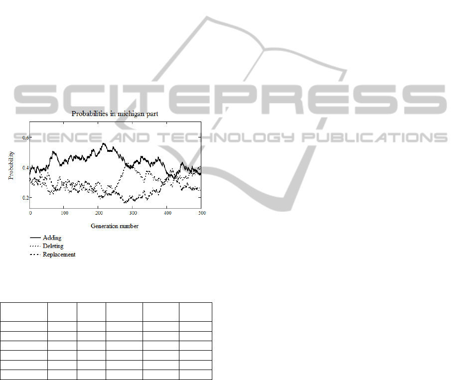
is shown in Figure 2. The graphs demonstrate the
change in the different Michigan operators’
probabilities during one of the runs. The testing was
performed for the Australian problem.
In the first stages, good fitness improvements can
be obtained by adding new rules to the base, so the
probability for adding increases as we can see and
the two others decrease. However, later, at about the
250
th
generation, the rule deleting operator becomes
as important as rule adding operator. At the stage of
about the 400
th
generation all three operators have
equal importance for a short time period, i.e. the
replacement operator receives resources back from
the other two. And, at the end of process, the
replacement operator again loses its importance. As
one can see, computational resources are actively
redistributed when the algorithm is executed.
Similar graphs can be obtained for the other
operator types.
Figure 2: Probabilities change during the algorithm run.
Table 5: Rule bases parameters.
Problem Learn Test
Number
of rules
Rule
length
Time
Australian 0.910 0.864 17,7 4,1 25.4s
German 0.801 0.748 22,3 5,3 48.9s
Segment 0.914 0.878 16,5 7,7 556s
Pageblocks 0.958 0.942 7,90 4,4 309s
Phoneme 0.830 0.807 12,2 2,7 313s
Satimage 0.843 0.822 27,8 16,6 822s
Also during the algorithm run the number of
rules in the best obtained solution, as well as the
average rule length, was captured. Table 3 contains
the averaged values of these parameters for all the
test problems. The number of rules is adjusted by the
algorithm and is different for every problem.
As an example, the rule base for the Pageblocks
(10 variables, 5 classes) problem is shown below. It
contains 7 rules with an average length of 5.28. The
learning accuracy with this rule base is 0.964, and
the testing accuracy is 0.959.
If X
1
is A
11
and X
3
is A
9
and X
6
is A
10
and X
8
is
A
3
then class 4 with weight 1;
If X
4
is A
4
and X
7
is A
7
and X
8
is A
3
then class 1
with weight 0.869;
If X
1
is A
2
and X
3
is A
10
and X
4
is A
1
and X
5
is
A
14
and X
6
is A
2
and X
8
is A
6
and X
9
is A
10
and
X
10
is A
6
then class 3 with weight 0.693;
If X
1
is A
11
and X
5
is A
6
and X
6
is A
3
and X
9
is
A
2
and X
10
is A
6
then class 4 with weight 0.775;
If X
1
is A
2
and X
2
is A
1
and X
4
is A
1
and X
5
is A
2
and X
6
is A
2
and X
7
is A
3
and X
8
is A
1
and X
9
is
A
3
and X
10
is A
6
then class 0 with weight 0.584;
If X
1
is A
1
and X
4
is A
2
and X
5
is A
3
and X
8
is A
1
and X
9
is A
2
then class 0 with weight 0.932;
If X
1
is A
1
and X
4
is A
6
and X
8
is A
13
then class
2 with weight 1.
6 CONCLUSIONS
In this paper, the self-configuring evolutionary
algorithm for automated design of fuzzy rule bases
was considered.
This method is much like the genetic algorithm,
which is often used to form fuzzy systems, but it has
the ability to adjust the number and the length of
rules, has special crossover and initialization
operators and the Michigan part. The Michigan part
of the algorithm allows accurate adjustment of rule
bases for the classification problem using
misclassified objects for building new rules. It also
deletes the rules that describe only a small part of
the sample to simplify the rule base. The algorithm
can find accurate and small rule bases quite quickly,
and its performance is comparable to other well-
known methods.
Further improvements of this approach may
include the use of multi-objective techniques and
some speed optimization.
ACKNOWLEDGEMENTS
This research is supported by the Ministry of
Education and Science of Russian Federation within
State Assignment № 2.1889.2014/K.
The authors express their gratitude to Mr.
Ashley Whitfield for his efforts to improve the text
of this article.
ICINCO2014-11thInternationalConferenceonInformaticsinControl,AutomationandRobotics
322

REFERENCES
Alcala R., Alcala-Fernandez J., Herrera F., Otero J.
Genetic learning of accurate and compact fuzzy rule
based systems based on the 2-tuples linguistic
representation, International Journal of Approximate
Reasoning 44. – 2007. – p. 45–64.
Alcalá-Fdez J., L. Sánchez, S. Garcia, M. J. del Jesus, S.
Ventura, J. M. Garrell, J. Otero, C. Romero, J.
Bacardit, V. M. Rivas, J. C. Fernández, and F. Herrera,
KEEL: A software tool to assess evolutionary
algorithms for data mining problems, Soft Comput.,
vol. 13, no. 3, pp. 307–318, Feb. 2009.
Asuncion A., D. Newman, 2007. UCI machine learning
repository. University of California, Irvine, School of
Information and Computer Sciences. URL:
http://www.ics.uci.edu/~mlearn/MLRepository.html.
Bodenhofer U., Herrera F. Ten Lectures on Genetic Fuzzy
Systems // Preprints of the International Summer
School: Advanced Control—Fuzzy, Neural, Genetic. –
Slovak Technical University, Bratislava. – 1997. p. 1–
69.
Cordon O., F. Herrera, F. Hoffmann and L.
Magdalena, Genetic Fuzzy Systems. Evolutionary
tuning and learning of fuzzy knowledge bases,
Advances in Fuzzy Systems: Applications and Theory,
World Scientific, 2001.
Fazzolari M., R. Alcalá, Y. Nojima, H. Ishibuchi, F.
Herrera, A Review of the Application of Multi-
Objective Evolutionary Fuzzy Systems: Current Status
and Further Directions. IEEE Transactions on Fuzzy
Systems, 21:1 (2013) 45-65.
Fernández A., Jesus M., Herrera F. Hierarchical fuzzy rule
based classification systems with genetic rule selection
for imbalanced data-sets International Journal of
Approximate Reasoning 50. – 2009. – p. 561–577.
Ishibuchi H., T. Yamamoto, Rule weight specification in
fuzzy rule-based classification systems, IEEE Trans.
Fuzzy Systems 13 (2005) 428–435.
Semenkin E., Semenkina M. Self-configuring Genetic
Algorithm with Modified Uniform Crossover Operator
// Y. Tan, Y. Shi, and Z. Ji (Eds.): Advances in Swarm
Intelligence. – Lecture Notes in Computer Science
7331. – Springer-Verlag, Berlin Heidelberg, 2012. –
P. 414-421.
Semenkin, E. S., Semenkina, M. E. The Choice of
Spacecrafts' Control Systems Effective Variants with
Self-Configuring Genetic Algorithm // Ferrier, J.L. et
al (Eds.): Informatics in Control, Automation and
Robotics: Proceedings of the 9th International
Conference ICINCO’2012. – Vol. 1. – Rome: Italy,
2012. – P. 84-93.
Semenkin E., Semenkina M. Stochastic Models and
Optimization Algorithms for Decision Support in
Spacecraft Control Systems Preliminary Design //
Informatics in Control, Automation and Robotics. -
Lecture Notes in Electrical Engineering, Volume 283.
– Springer-Verlag, Berlin Heidelberg, 2014. – P. 51-
65.
L. X. Wang, J. M. Mendel, Generating fuzzy rules by
learning from examples, IEEE Transactions on
Systems, Man, and Cybernetics 22:6 (1992) 1414-
1427.
FuzzyRuleBasesAutomatedDesignwithSelf-configuringEvolutionaryAlgorithm
323
