
Closing the Loop on a Complete Linkage Hierarchical Clustering Method
David Allen Olsen
Department of Computer Science and Engineering, University of Minnesota-Twin Cities, Minneapolis, U.S.A.
Keywords:
Intelligent Control Systems, Hierarchical Clustering, Hierarchical Sequence, Complete Linkage, Meaningful
Level, Meaningful Cluster Set, Distance Graphs.
Abstract:
To develop a complete linkage hierarchical clustering method that 1) substantially improves upon the accu-
racy of the standard complete linkage method and 2) can be fully automated or used with minimal operator
supervision, the assumptions underlying the standard complete linkage method are unwound, evaluating pairs
of data points for linkage is decoupled from constructing cluster sets, and cluster sets are constructed de
novo. These design choices make it possible to construct only the cluster sets that correspond to select, pos-
sibly non-contiguous levels of an
n·(n−1)
2
+ 1-level hierarchical sequence. To construct meaningful cluster
sets without constructing an entire hierarchical sequence, a means that uses distance graphs is used to find
meaningful levels of such a hierarchical sequence. This paper presents an approach that mathematically cap-
tures the graphical relationships that are used to find meaningful levels and integrates the means into the new
clustering method. The approach is inexpensive to implement. Consequently, the new clustering method is
self-contained and incurs almost no extra cost to determine which cluster sets should be constructed and which
should not. Empirical results from four experiments show that the approach does well at finding meaningful
levels of hierarchical sequences.
1 INTRODUCTION
This paper presents the third part of a three-part re-
search project and is a companion paper to Means
for Finding Meaningful Levels of a Hierarchical
Sequence Prior to Performing a Cluster Analysis
(Olsen, 2014b). The goal of this project was to de-
velop a general, simplistic, complete linkage hier-
archical clustering method that 1) substantially im-
proves upon the accuracy of the standard complete
linkage method and 2) can be fully automated or used
with minimal operator supervision. It was motivated
by the need to bring machine learning, and complete
linkage hierarchical clustering in particular, over from
the “computational side of things ... to the system
ID/model ID kind of thinking” (Gill, 2011) as part of
closing the loop on cyber-physical systems.
For the first part of the project, a new, complete
linkage hierarchical clustering method was devel-
oped. See (Olsen, 2014a). The new clustering method
is consonant with the model for a measured value that
scientists and engineers commonly use
1
, so it sub-
1
The model for a measured value is measured value =
true value + bias (accuracy) + random error (statistical un-
certainty or precision) (Navidi, 2006). This model has sub-
stantially improves upon the accuracy of the standard
complete linkage method. Further, it can construct
cluster sets for select, possibly non-contiguous levels
of an
n·(n−1)
2
+1-level hierarchical sequence. The new
clustering method was designed with small-n, large-
m data sets in mind, where n is the number of data
points, m is the number of dimensions, and “large”
means thousands and upwards (Murtagh, 2009).
2
Because the computational power presently ex-
ists to apply hierarchical clustering methods to much
larger data sets than when the standard complete
linkage method was developed, the new clustering
method unwinds the assumptions that underlie the
standard complete linkage method. However, by un-
winding these assumptions and letting the size of a
stantially broader applicability than the taxonomic model
that is the basis for the standard complete linkage method.
2
These data sets are used by many cyber-physical sys-
tems and includes time series. For example, a typical au-
tomobile has about 500 sensors; a small, specialty brewery
has about 600 sensors; and a small power plant has about
1100 sensors. The new clustering method may accommo-
date large-n, large-m data sets as well, and future work in-
cludes using multicore and/or heterogeneous processors to
parallelize parts of the new clustering method, but large-n,
large-m data sets are not the focus here.
296
Allen Olsen D..
Closing the Loop on a Complete Linkage Hierarchical Clustering Method.
DOI: 10.5220/0005058902960303
In Proceedings of the 11th International Conference on Informatics in Control, Automation and Robotics (ICINCO-2014), pages 296-303
ISBN: 978-989-758-039-0
Copyright
c
2014 SCITEPRESS (Science and Technology Publications, Lda.)
hierarchical sequence revert back from n levels to
n·(n−1)
2
+ 1 levels, the time complexity to construct
cluster sets becomes O(n
4
). This is large even for
small-n, large-m data sets. Moreover, the post hoc
heuristics for cutting dendrograms are not suitable for
finding meaningful cluster sets
3
of an
n·(n−1)
2
+ 1-level
hierarchical sequence.
Thus, with today’s technology, the project went
back more than 60 years to solve a problem that could
not be solved then. For the second part of the project,
a means was developed for finding meaningful lev-
els of an
n·(n−1)
2
+ 1-level (complete linkage) hierar-
chical sequence prior to performing a cluster analy-
sis. The means constructs a distance graph
4
and vi-
sually examines this graph for features that correlate
with the meaningful levels. (Olsen, 2014b). By find-
ing meaningful levels of such a hierarchical sequence
prior to performing a cluster analysis, it is possible
to know which cluster sets to construct and construct
only these cluster sets.
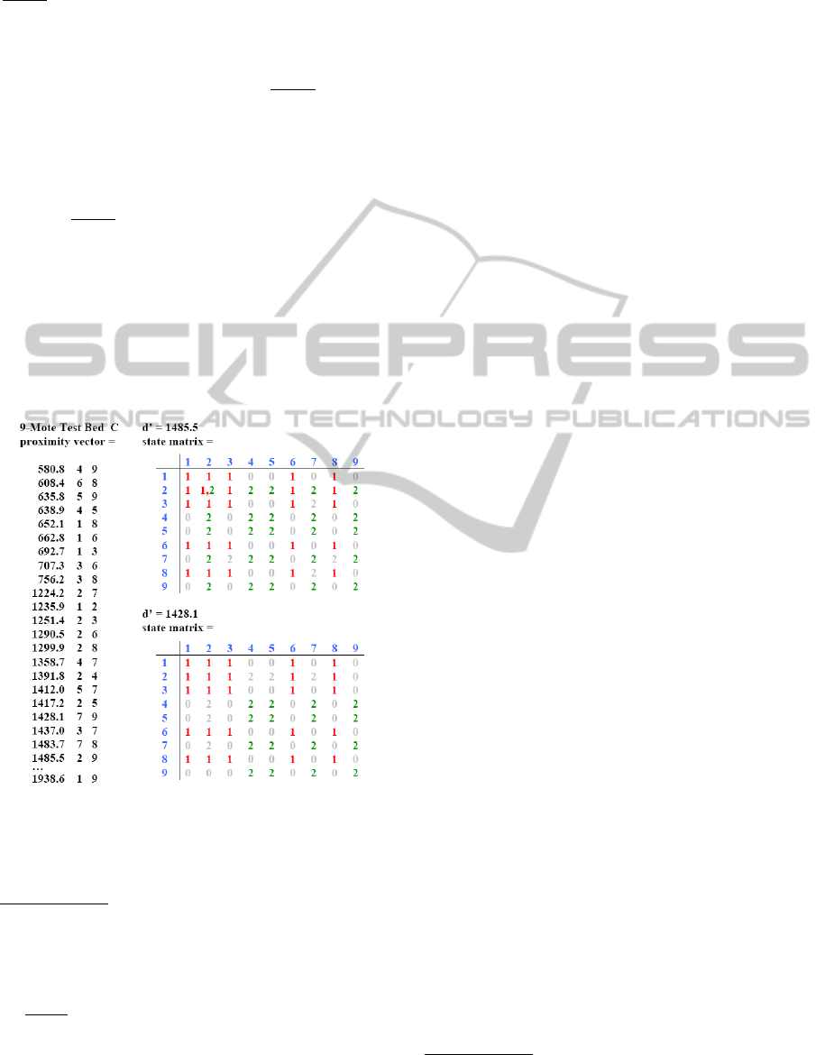
Figure 1: Proximity vector and state matrices for a data set
similar to that described in Subsection 5.2. The numbers
in the state matrices highlight the different clusters and are
for illustrative purposes only. How these data structures are
used is fully described in (Olsen, 2014a).
3
A “meaningful cluster set” refers to a cluster set that
can have real world meaning. Under ideal circumstances,
a “meaningful level” refers to a level of a hierarchical se-
quence at which a new configuration of clusters has fin-
ished forming. These definitions appear to be synonymous
for
n·(n−1)
2
+ 1-level hierarchical sequences. The cluster set
that is constructed for a meaningful level is a meaningful
cluster set, so these terms are used interchangeably.
4
Examples of distance graphs can be found in Fig. 2 and
the experiments in Section 5.
This reduces the time complexity to construct
cluster sets from O(n
4
) to O(ln
2
), where l is the num-
ber of meaningful levels. These are the cluster sets
that can have real world meaning. It is notable that
the means does not rely on dendrograms or post hoc
heuristics to find meaningful cluster sets. The second
part also looked at how increasing the dimensional-
ity of the data points helps reveal inherent structure in
noisy data, which is necessary for finding meaningful
levels.
The third part of the project resolved how to math-
ematically capture the graphical relationships that un-
derlie the above-described features and integrate the
means into the new clustering method. By doing
so, the new clustering method becomes self-contained
and can be fully automated or used with minimal op-
erator supervision.
2 CONSTRUCTING SELECT
CLUSTER SETS
Let X = {x
1
,x
2
,...,x
n
} be a data set that contains a
finite number of data points n, where each data point
has m dimensions. Further, suppose that each data
point is a sequence of samples and that at any mo-
ment in time, with respect to each class or source, all
the samples have the same true values and biases
5
.
The INCLude (InterNodal Complete Linkage) hierar-
chical clustering method (Olsen, 2014a) is a complete
linkage hierarchical clustering method that assumes
only that the clusters are globular or compact, and
preferably maximally complete subsets of data points.
It uses interpoint distances instead of intercluster dis-
tances to construct clusters, allows clusters to overlap,
and allows data points to migrate between clusters.
Unlike the standard complete linkage method, or
the clique detection method described in (Peay, 1974)
and (Peay, 1975), the new clustering method is not
an updating method. Instead, as Fig. 1 shows, the
new clustering method substitutes two data structures,
a proximity vector for holding information about the
distances between the data points and a state matrix
for holding information about linkage, for the prox-
imity matrix used by the standard complete linkage
method. In particular, a proximity vector is a rank
ordered list of ordered triples (d
i, j
,i, j) comprised of
a distance d
i, j
between data points x
i
and x
j
, i, j =
1,2,...,n,i 6= j, and the indices of the respective data
points. The ordered triples are sorted into rank or as-
cending order according to their distance elements,
5
In real world terms, this is the same as calibrating the
sensors.
ClosingtheLooponaCompleteLinkageHierarchicalClusteringMethod
297

and the row indices of the proximity vector are used
to index the sorted ordered triples (the “rank order in-
dices”).
Next, the ordered triples are evaluated in ascend-
ing order for linkage. As the ordered triples are evalu-
ated, threshold distance (index) d
0
increases implicitly
from 0 to the maximum of all the distance elements.
Threshold distance d
0
∈ R is a continuous variable
that determines which pairs of data points in a data
set are linked and which are not. Data points x
i
and
x
j
, i, j = 1,2,...,n,i 6= j, are linked if the distance be-
tween them is less than or equal to threshold distance
d
0
, i.e., d
i, j
≤ d
0
. From the linkage information that is
stored in the state matrix and the degrees of the data
points, a hierarchical sequence of cluster sets is con-
structible.
Because evaluating ordered triples for linkage is
decoupled from cluster set construction, the linkage
information in a state matrix can be updated without
constructing cluster sets. Further, cluster sets are con-
structed de novo. In other words, the cluster set for
each level of an
n·(n−1)
2
+1-level hierarchical sequence
is constructed independently of the cluster sets for the
other levels. This scheme has at least two advantages.
First, data points can migrate naturally as a part of
cluster set construction. Second, it is possible to con-
struct only the cluster sets that correspond to select,
possibly non-contiguous levels of a hierarchical se-
quence. Consequently, it is possible to construct only
the cluster sets for meaningful levels of a hierarchical
sequence.
3 USING DISTANCE GRAPHS TO
FIND MEANINGFUL LEVELS
To find meaningful levels of an
n·(n−1)
2
+ 1-level hi-
erarchical sequence, a distance graph is constructed
and visually examined. For 2-norm distance measures
such as Euclidean distance, using distance graphs is
motivated by the realization that as m → ∞, the vari-
ance σ
2
Z
m
of the random variable Z
m
= (
∑
m
k=1
Y
2
k
)
1
2
converges to
∑
m
k=1
σ
4
k
2(
∑
m
k=1
σ
2
k
+
∑
m
k=1
µ
2
k
)
+
∑
m
k=1
σ
2
k
µ
2
k
∑
m
k=1
σ
2
k
+
∑
m
k=1
µ
2
k
.
6
Y
k
is a normally distributed random variable such that
Y
k
∼ N(µ
k
,σ
k
). Often, as the dimensionality of the
data points increases and the 2-norm interclass dis-
tances become larger, the standard deviations of the
2-norm interclass distances, i.e., σ
Z
m
, nonetheless re-
main relatively small or constant. See (Olsen, 2014b).
When this scenario holds, data points that belong
6
An analog exists for 1-norm distance measures such as
city block distance.
to the same class link at about the same time even at
higher dimensionalities. Classes of data points can be
close together at lower dimensionalities. When they
are, the magnitudes of many intraclass distances and
interclass distances are about the same, so the two
kinds of distances commingle. However, the classes
of data points are farther apart at higher dimensional-
ities, so the intraclass distances and the interclass dis-
tances segregate into bands. Thus, higher dimension-
alities can attenuate the effects of noise
7
that preclude
finding meaningful levels of a hierarchical sequence
at lower dimensionalities and distinguish between the
classes. Moreover, this pattern repeats itself as clus-
ters become larger from including more data points.
Consequently, as the dimensionality of the data
points increases, the distance graphs for a data set
can exhibit identifiable features that correlate with
meaningful levels of the corresponding hierarchical
sequences. These levels are the levels at which multi-
ple classes have finished linking to form new config-
urations of clusters. In particular, assuming that the
data set has inherent structure, a distance graph takes
on a shape whereby sections of the graph run nearly
parallel to one of the graph axes. Where there is very
little or no linking activity, the sections run nearly ver-
tically. Where there is significant activity, i.e., where
new configurations of clusters are forming, the sec-
tions run nearly horizontally. Thus, portions of the
graph that come after the lower-right corners and be-
fore the upper-left corners indicate where new config-
urations of clusters have finished forming. A distance
graph can be visually examined prior to performing a
cluster analysis. Since a distance graph is used to find
meaningful levels of a hierarchical sequence prior to
performing a cluster analysis, it is not a summary of
the results obtained from the analysis. Instead, it en-
ables a user to selectively construct only meaningful
cluster sets, i.e., cluster sets where new configurations
of clusters have finished forming.
Finding meaningful levels is remarkably easy:
First, the differences (dissimilarities) between data
points x
i
and x
j
, i, j = 1, 2,..., n,x
i
6= x
j
, are calcu-
lated. Then, using a p-norm, p ∈ [1,∞), the lengths
or magnitudes of the vectors that contain these differ-
ences are calculated. Next, ordered triples (d
i, j
,i, j)
are constructed from these distances and the indices
of the respective data points, the ordered triples are
sorted into rank or ascending order according to their
distance elements, and rank order indices are assigned
to the sorted ordered triples. The rank order indices
and the ordered triples are used to construct a distance
graph. The rank order indices and/or the distance el-
7
Attenuating the effects of noise refers to reducing the
effects of noise on cluster construction.
ICINCO2014-11thInternationalConferenceonInformaticsinControl,AutomationandRobotics
298
ements that correspond to where the lower-right cor-
ners appear in the graph are identified along the axes
of the distance graph. These rank order indices and
distance elements coincide with the meaningful lev-
els and the respective threshold distances d
0
of the
corresponding hierarchical sequence. Each different
distance measure has its own distance graph and cor-
responding hierarchical sequence, and thus its own set
of meaningful levels. As a visual tool, however, dis-
tance graphs are not well suited for automation.
4 INTEGRATING THE MEANS
Integrating the means for finding meaningful levels
into the new clustering method is based on the same
two assumptions that underlie the means when dis-
tance graphs are visually examined. First, the ap-
proach assumes that noise (random error) is the only
random component in a measured value and that the
noise that is embedded in each dimension (sample) of
each data point is statistically independent.
8
Second,
the approach assumes that the dissimilarities between
the data points are non-negative values. This assump-
tion is needed because p-norm distance measures do
not distinguish between positive and negative correla-
tion.
To mathematically capture the graphical relation-
ships that underlie the above-described features of a
distance graph, the rank order indices that coincide
with the meaningful levels of the corresponding hier-
archical sequence, or the distance elements that coin-
cide with the respective threshold distances d
0
, must
be identifiable without visually examining the dis-
tance graph. In other words, this objective must be
attainable by looking only at the rank order indices
and the information that is contained within the or-
dered triples. As mentioned above, those portions of a
distance graph that come after the lower-right corners
and before the upper-left corners indicate where new
configurations of clusters have finished forming. The
approach focuses on the lower-right corners because,
under ideal circumstances, these are the features that
correspond to having evaluated every ordered triple
whose distance element is less than threshold distance
d
0
. As Fig. 2 shows, one way to mathematically cap-
ture these relationships compares 1) the tangent of the
angle that the distance graph forms with the x-axis of
8
To make the proofs mathematically tractable, the work
on finding meaningful levels also assumed that noise can be
modeled as Gaussian random variables. When noise is uni-
formly distributed, the results are analogous to those when
noise is normally distributed, indicating that the Gaussian
random variable assumption is reasonable (Olsen, 2014b).
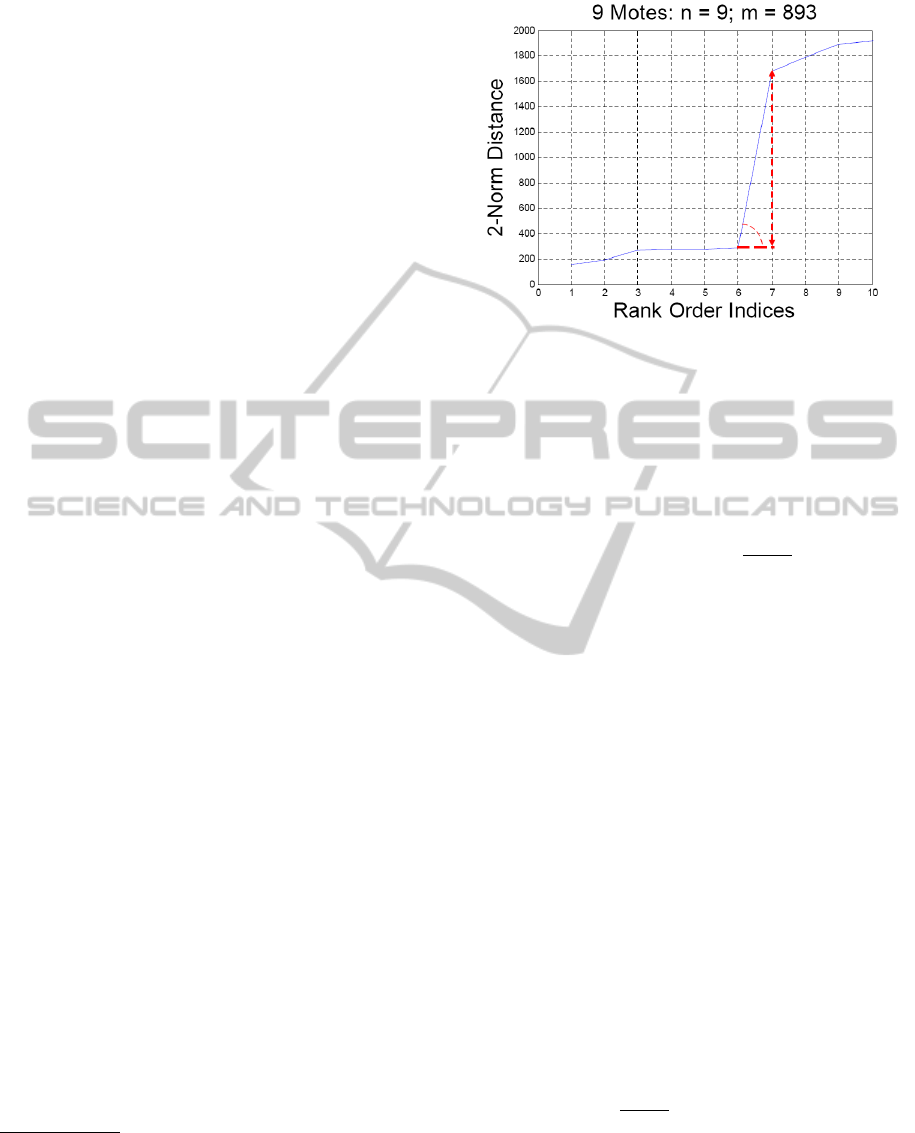
Figure 2: Lower left portion of the distance graph from the
experiment in Subsection 5.2. The enlargement shows one
of the angles used to find meaningful levels of the corre-
sponding hierarchical sequence. The dashed arrow repre-
sents DIST ROI
i+1
− DIST ROI
i
. Here, DIST ROI
i+1
is the
distance element of the 7th ordered triple and DIST ROI
i
is
the distance element of the 6th ordered triple.
the graph at each rank order index i with 2) the dif-
ference between the distance elements of the i + 1th
and ith ordered triples, i = 1, 2,...,
n·(n−1)
2
. The experi-
ments in Section 5 show that the range of these angles
typically is between 60 degrees and 90
−
degrees, or
nearly orthogonal under ideal circumstances.
Proximity vectors are well suited for finding these
angles. With respect to a specific distance measure,
a proximity vector is a permanent record of the
interpoint distances between the data points in a data
set. After each ordered triple is evaluated for linkage,
a test is performed to determine whether the next
level of the corresponding hierarchical sequence is
meaningful. The ith level of a hierarchical sequence
is deemed to be meaningful if the following test
returns true:
DIST ROI
i+1
− DIST ROI
i
≥ tan(cuto f f Angle) ·
MAXDIST /MAXROI.
DIST ROI
i+1
is the distance element of the i + 1th
ordered triple, DIST ROI
i
is the distance element of
the ith ordered triple, cuto f f Angle is the minimum
angle that the distance graph must form with the
positive x-axis of the graph at the ith rank order
index, MAX DIST is the maximum distance element,
and MAXROI is
n·(n−1)
2
or the number of ordered
triples. The normalization factor is on the right side
of the equation to reduce the number of multipli-
cations. Typically, a distance graph is constructed
and examined before any of the ordered triples are
evaluated for linkage. The test is performed after
each ordered triple is evaluated. If the test returns true
ClosingtheLooponaCompleteLinkageHierarchicalClusteringMethod
299

after the ith ordered triple is evaluated, the cluster
set for the ith level of the hierarchical sequence is
constructed. The first cluster set (all the data points
are singletons) and the last cluster set (all the data
points belong to the same cluster or stopping criteria
have been met) are always constructed.
Two parameters need tuning. One is the dimen-
sionality at which inherent structure in a data set has
good definition (or as good as is practically possible).
The other is cuto f f Angle. These can be tuned on-
line with minimal operator intervention or hardwired
based on domain knowledge. Alternatively, it should
be possible to learn them. The results for a data set
can be characterized by the data set and the index
m(∠cuto f f Angle), where m is the dimensionality of
the data points.
5 EMPIRICAL RESULTS
The remainder of this paper describes the empirical
results from four experiments that were rerun to eval-
uate the above-described approach. The original ex-
periments are part of the work described in (Olsen,
2014a) and (Olsen, 2014b). In all four experiments,
the approach is used to find meaningful levels of hier-
archical sequences. These results are compared with
those obtained from visually examining the corre-
sponding distance graphs. Defining false positives
to mean meaningful levels that should not be con-
structed but are and false negatives to mean meaning-
ful levels that should be constructed but are not, the
third experiment also calculates the number of false
positives and false negatives as the dimensionality of
the data set is increased. The fourth experiment looks
at the ranges over which cuto f f Angle can vary with-
out incurring any false positives or false negatives.
Both the 2-norm distance measure (Euclidean dis-
tance) and the 1-norm distance measure (city block
distance) are used to calculate the distances. level
is a variable that is used to refer to individual mean-
ingful levels, and d
0
refers to the respective threshold
distances d
0
. Before the means was integrated, the
new clustering method was compared with the stan-
dard complete linkage method and a flat method in
(Olsen, 2014a).
5.1 No Structure
A uniform distribution pseudo-random number gener-
ator is used to construct 100 data points having 10,000
dimensions each. Out of 4951 levels in total, the
graphs in Fig. 3 suggest that the corresponding hi-
erarchical sequences have no meaningful levels other
than the end levels. The data for the 2-norm distance
measure include 9 false positives at 10K(∠60), 9 false
positives at 10K(∠65), 3 false positives at 10K(∠70),
3 false positives at 10K(∠75), 1 false positive at
10K(∠80), and no false positives at 10K(∠85). The
data for the 1-norm distance measure include 6 false
positives at 10K(∠60), 5 false positives at 10K(∠65),
5 false positives at 10K(∠70), 3 false positives at
10K(∠75), 1 false positive at 10K(∠80), and no false
positives at 10K(∠85). The false positives come at
either end of the hierarchical sequences for both dis-
tance measures.
5.2 Sampling Luminescence
Nine Crossbow
R
MicaZ motes with MTS300CA
sensor boards attached thereto are configured into a
1x1 meter grid and programmed to take light read-
ings (lux) of an overhead light source every 1 second
for 15 minutes. Canopies are placed over some of the
motes during part or all of the experiment. Out of
37 levels in total, the graphs in Fig. 4 suggest that
the corresponding hierarchical sequences have four
meaningful levels. At level = 6 (d
0
= 287.97 for the
2-norm distance measure and d
0
= 6723.20 for the 1-
norm distance measure; m = 893), there are five non-
overlapping clusters, one for motes that are always
exposed to direct light (motes 2, 4, and 9), another
for motes that are never exposed to direct light (motes
1, 6, and 8), and one for each of the motes that are
exposed to direct light during different time intervals
(motes 3, 5, and 7). At level = 27 (d
0
= 2488.63 for
the 2-norm distance measure and d
0
= 64,391.60 for
the 1-norm distance measure; m = 893), there are two
overlapping clusters, one for those motes that were
exposed to direct light during part or all of the exper-
iment (motes 2, 3, 4, 5, 7, and 9) and the other for
those motes that were not exposed to direct light dur-
ing part or all of the experiment (motes 1, 3, 5, 6, 7,
and 8).
The meaningful levels of the hierarchical se-
quence for the 2-norm distance measure are identi-
fiable from 893(∠60) to 893(∠70). At 893(∠65) and
893(∠70), the meaningful levels are identifiable with-
out incurring any false positives or false negatives.
The meaningful levels of the hierarchical sequence
for the 1-norm distance measure are identifiable from
893(∠60) to 893(∠80). At 893(∠80), the meaning-
ful levels are identifiable without incurring any false
positives or false negatives.
ICINCO2014-11thInternationalConferenceonInformaticsinControl,AutomationandRobotics
300
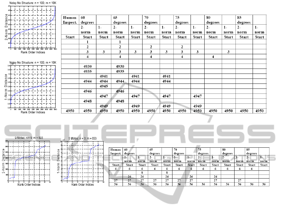
Figure 3: Distance graphs for the structureless data set at m = 10,000 dimensions and levels identified as meaningful for
10K(∠60) to 10K(∠85).
Figure 4: Distance graphs for the nine motes data set at m = 893 dimensions and levels identified as meaningful for 893(∠60)
to 893(∠85).
5.3 17-Point Geometric Pattern
As shown in Fig. 5, a 17-point geometric pattern is
constructed, and five copies of each point are used to
construct a data set having 85 data points. The di-
mensionality of the data points is increased to 80,000
dimensions by increments of 10,000 dimensions, and
noise (N(0,2
2
)) is added to each dimension of each
data point in each data set. The graphs in Fig. 5 sug-
gest that the hierarchical sequence for the 2-norm dis-
tance measure has 19 meaningful levels while that for
the 1-norm distance measure has 16 levels. These lev-
els are provided in (Olsen, 2014a).
This experiment compares how many false pos-
itives and how many false negatives are incurred at
different dimensionalities. As the table in Fig. 5
shows, except when cuto f f Angle equals 80 or 85 de-
grees, the number of false positives is greater than
the number of false negatives. Most false positives
are levels of the hierarchical sequences just to either
side of the meaningful levels. More false positives
occur at lower dimensionalities, most likely due to
noise, and at lower cuto f f Angles, because the crite-
rion for constructing cluster sets is less stringent. If
they occur, false negatives tend to occur at very high
cuto f f Angles or at lower dimensionalities, where the
definition of the meaningful levels is not as good as
it is at higher dimensionalities. From 70K(∠75) to
80K(∠85), there are no false positives or false nega-
tives.
5.4 Health Monitoring
The data used in this experiment come from file
16265 of the MIT-BIH PhysioNet Normal Sinus
Rhythm database (Goldberger et al., 2000). This file
contains ECG readings collected at 128 hertz. The
P,Q,R,S,T interval of each heart beat, as illustrated by
the left-most graphs in Fig. 6, describes how a heart
pumps blood to other parts of a body. Here, 25 sam-
ples per beat that include the Q,R,S complex and at
least the left side of the ST element are extracted from
the first 300 consecutive beats of the file, and the data
set is divided into 10 segments (approx. 25 seconds
each). The third graph in Fig. 6 shows that this data
set has almost no inherent structure.
An elevated ST element is simulated by adding
a constant c
elevST
equal to 80, 100, or 150 mV to
samples 11-22 of the excerpts in the last 1, 2, 3, 4,
or 5 segments. This experiment looks at how early
ClosingtheLooponaCompleteLinkageHierarchicalClusteringMethod
301
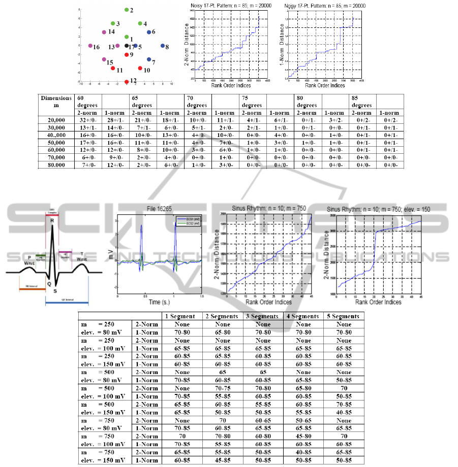
Figure 5: 17-point geometric pattern, distance graphs for the 17-point geometric pattern data set at m = 20,000 dimensions,
and false positives (+) and false negatives (-) for 20K(∠60) to 80K(∠85).
Figure 6: ECG, distance graphs for m = 750 dimensions, and ranges over which cuto f f Angle can vary without incurring
any false positives or false negatives. The data used in this experiment come from file 16265 of the MIT-BIH Normal Sinus
Rhythm database.
an elevated ST element is detectable without incur-
ring any false positives or false negatives. Increas-
ing c
elevST
or increasing the dimensionality of the
segments increases the ranges of cuto f f Angle over
which an event is detectable. Increasing c
elevST
adds
structure to the data sets and has the biggest impact
on the ranges over which an event is detectable. In-
creasing the dimensionality of the segments does not
add structure to the data sets, and the law of dimin-
ishing returns eventually sets in. The widest ranges of
detection are where both c
elevST
and m are large. The
number of segments to which c
elevST
is added does not
show a clear trend. This is consistent with the view
that increasing or decreasing the number of segments
should not have an effect on the ranges. For this ex-
periment, the ranges for the 1-norm distance measure
tend to be wider than those for the 2-norm distance
measure.
ICINCO2014-11thInternationalConferenceonInformaticsinControl,AutomationandRobotics
302

6 CONCLUSION
To develop a complete linkage hierarchical clustering
method that 1) substantially improves upon the accu-
racy of the standard complete linkage method and 2)
can be fully automated or used with minimal opera-
tor supervision, the assumptions underlying the stan-
dard complete linkage method are unwound. The new
clustering method substitutes two data structures, a
proximity vector and a state matrix, for the proximity
matrix used by the standard complete linkage method.
Consequently, evaluating pairs of data points for link-
age is decoupled from constructing cluster sets. Fur-
ther, cluster sets are constructed de novo. These de-
sign choices make it possible to construct only the
cluster sets that correspond to select, possibly non-
contiguous levels of an
n·(n−1)
2
+ 1-level hierarchical
sequence. To construct meaningful cluster sets with-
out constructing an entire hierarchical sequence, a
means that uses distance graphs is used to find mean-
ingful levels of such a hierarchical sequence.
This paper presents an approach that mathemati-
cally captures the graphical relationships that are used
to find meaningful levels and integrates the means
into the new clustering method. The test that deter-
mines which cluster sets are meaningful is easy to cal-
culate and uses the same data that are used by the new
clustering method. Consequently, the new clustering
method is self-contained and incurs almost no extra
cost to administer the test after each ordered triple is
evaluated. Moreover, the approach is adaptable and
broadly applicable because it does not rely on prede-
termined parameters. Future work includes trying the
new clustering method at a beta site and making en-
hancements to the cluster set construction module.
The empirical results from four experiments show
that the approach does well at finding meaningful lev-
els of hierarchical sequences. Most false positives are
levels just to either side of the meaningful levels. The
results also show that it is possible to identify mean-
ingful levels of a hierarchical sequence without incur-
ring any false positives or false negatives.
ACKNOWLEDGEMENTS
The author thanks Dr. John Carlis, Department of
Computer Science and Engineering, University of
Minnesota, for his general guidance and advice on
technical writing. The author also thanks the paper’s
reviewers for reviewing the paper and for their helpful
feedback.
REFERENCES
Gill, H. (2011). CPS overview. In Symposium on
Control and Modeling Cyber-Physical Sys-
tems (www.csl.illinois.edu/video/csl-emerging-
topics-2011-cyber-physical-systems-helen-gill-
presentation), Champaign, IL.
Goldberger, A., Amaral, L., Glass, L., Hausdorff,
J., Ivanov, P., Mark, R., Mietus, J., Moody,
G., Peng, C., and Stanley, H. (June 13, 2000).
PhysioBank, PhysioToolkit, and PhysioNet:
Components of a New Research Resource
for Complex Physiologic Signals. Circulation
101(23):e215-e220 [Circulation Electronic Pages;
http://cir.ahajournals.org/cgi/content/full/101/
23/e215].
Murtagh, F. (2009). The remarkable simplicity of very high
dimensional data: Application of model-based clus-
tering. J. of Classification, 26:249–277.
Navidi, W. (2006). Statistics for Engineers and Scientists.
McGraw-Hill.
Olsen, D. (2014a). Include hierarchical clustering: A hier-
archical clustering method based solely on interpoint
distances. Technical report, Minneapolis, MN.
Olsen, D. (2014b). Means for finding meaningful lev-
els of a hierarchical sequence prior to performing a
cluster analysis. In Proceedings of the 11th Interna-
tional Conference on Informatics in Control, Automa-
tion and Robotics (ICINCO 2014), Vienna, Austria.
Peay, E. (1974). Hierarchical clique structures. Sociometry,
37(1):54–65.
Peay, E. (1975). Nonmetric grouping: Clusters and cliques.
Psychometrika, 40(3):297–313.
ClosingtheLooponaCompleteLinkageHierarchicalClusteringMethod
303
