
Input and State Constrained Nonlinear Predictive Control
Application to a Levitation System
Joanna Zietkiewicz
Institute of Control and Information Engineering, Poznan University of Technology, Piotrowo 3a, 60-965 Poznan, Poland
Keywords:
Predictive Control, Linear Quadratic Control, Feedback Linearization, Nonlinear Control.
Abstract:
The subject of the article concerns a constrained predictive control with feedback linearization (FBL) applied
for multiple-input and multiple-output (MIMO) system. It relies on finding a compromise in every step be-
tween feasible and optimal linear quadratic (LQ) control by minimization of one variable. Behaviour of model
signals in function of minimized variable is investigated, in order to assure the optimality of the solution. LQ
control based applications for feedback linearized models do not meet the problem of choosing weights in
linear quadratic cost function. That important problem is solved here by comparison of the cost function with
that obtained for the linear approximated system in the operating point. That provides satisfactory behaviour
and also justifies the simplified approach relied on minimization of only one variable for MIMO system.
1 INTRODUCTION
Feedback linearization method (Isidori, 1995),
(Khalil, 2002) as the exact method for linearizing
nonlinear models provides the advantage of possibil-
ity of using the linear control theory for nonlinear
systems. The LQ control is applied in the interpola-
tion method, proposed in (Poulsen et al., 2001). The
method allows us to introduce constraints of variables
into control designing. The advantage of this method
is that it relies on minimization of only one variable. It
was shown, that the method can be used for multiple-
input, multiple-output systems, providing that certain
conditions are fulfilled (Zietkiewicz, 2012).
Additional problem appears for feedback lin-
earizated models and linear quadratic control and it
concerns weights values in LQ cost function for feed-
back linearized model. In general the signals in the
cost function are not described by direct physical val-
ues. Experimental choice or methods involving val-
ues of variables like Bryson rule (Kang et al., 2014)
may not be sufficient. Usually in literature only
weights on diagonal are used and the part which pe-
nalizes functions of multiplied state and input vari-
ables is omitted. In (Poulsen et al., 2001) a constant
value was used in designing control to maintain the
equilibrium between values in cost function. It was
sufficient for given system, but in general equilibrium
between every state and input signals has to be con-
sider. The problem is solved in the article by using
cost function with signals of original nonlinear model
(it can be assumed as the cost function for the model
linearized in the operating point). Signals in that func-
tion are known as physical values and weights in it is
easier to choose. The function is rearranged by ap-
proximation of nonlinear dependencies between sig-
nals from nonlinear model and feedback linearized
model. The dependencies are obtained from feedback
linearization procedure. The finally obtained weights
in cost function for feedback linearized model assures
the equilibrium between variables of the model.
As the example to present the results of the
method, model of levitation system is used (mls2em,
2009). Problem of levitation control is the sub-
ject of many papers. Many types of control method
have been used, including backstepping technique
(Yang and Tateishi, 2001), sliding mode control (Al-
Muthairi and Zribi, 2004), fuzzy logic control (Ah-
mad et al., 2010), predictive control (Bachle et al.,
2013) with many others ideas and also fusions of
methods. The problem is still widely researched,
however only part of solutions consider constraints.
The model of levitation system used in this paper is
well described with basic control results in (Dragos
et al., 2012).
Simulations of proposed method for the levita-
tion model (mls2em, 2009) was performed in matlab
environment. Results show that signals fulfill con-
straints and appropriately chosen weight values cause
fast performance. The result of FBL application to
274
Zietkiewicz J..
Input and State Constrained Nonlinear Predictive Control - Application to a Levitation System.
DOI: 10.5220/0005055502740279
In Proceedings of the 11th International Conference on Informatics in Control, Automation and Robotics (ICINCO-2014), pages 274-279
ISBN: 978-989-758-039-0
Copyright
c
2014 SCITEPRESS (Science and Technology Publications, Lda.)

m
F
1
F
2
+ F
g
u
1
,x
3
u
2
,x
4
x
1
Figure 1: levitation system.
MIMO model is the decomposition to several linear
models. The maintained equilibrium between values
in cost functions of those linear models provides also
equilibrium in the influence of minimized variable on
that models. That justifies also the ability of the use
of only one minimized variable for MIMO systems.
2 LEVITATION SYSTEM
The object of control is the levitation system shown in
figure 1. It consists of two electromagnets and a ball
placed beetween them.
The dynamics of the object can be represented by
equations
˙x
1
= x
2
˙x
2
= −
F
emP1
mF
emP2
x
2
3
e
−
x
1
F
emP2
+ g+
F
emP1
mF
emP2
x
2
4
e
−
x
d
−x
1
F
emP2
˙x
3
=
f
iP2
f
iP1
(k
i
u
1
+ c
i
− x
3
)e
x
1
f
iP2
˙x
4
=
f
iP2
f
iP1
(k
i
u
2
+ c
i
− x
4
)e
x
d
−x
1
f
iP2
(1)
where: x
1
[m]- position of the ball, x
2
[m/s]- velocity
of the ball, x
3
,x
4
[A] - currents of the upper and lower
magnets coils respectively, u
1
,u
2
are the unitless con-
trol signals. The values of constants are presented in
table 1.
Table 1: Constant values of the levitation system.
parameter value description
m = 0.0571 kg ball mass
g = 9.81 m/s
2
gravity constant
F
emP1
= 1.7521∗ 10
−2
H electromagnet parameter
F
emP2
= 5.8231∗ 10
−3
H electromagnet parameter
f
iP1
= 1.4142∗ 10
−4
ms actuator parameter
f
iP2
= 4.5626∗ 10
−3
m actuator parameter
k
i
= 2.5165 A actuator parameter
c
i
= 0.0243 A actuator parameter
d = 0.075 m distance
b
d
= 0.06 m ball diameter
x
d
= 0.015 m d − b
d
Several variables in the system should restrict
given constraints:
0 m ≤ x
1
(t) ≤ x
d
m
0.03884 A ≤ x
3
(t),x
4
(t) ≤ 2.38 A
0.00498 ≤ u
1
(t),u
2
(t) ≤ 1
(2)
The objective of control is to shift the ball from
one given point to another by the use of control sig-
nals u
1
,u
2
with the restricion of constraints.
2.1 Feedback Linearization
For the output y = x
1
system has releative degre l = 3
and the dimmension of state space model is 4. Feed-
back linearization can be performed for square MIMO
models, with the same number, n, of inputs and out-
puts. In considered model there are two control inputs
and only one output. Additional output has to be cho-
sen; for the variable x
4
as output relative degree is
l
2
= 1. In this way sum of relative degrees equals the
model dimmension, therefore this variable is chosen
as the second output y
2
= x
4
.
Basic method for obtaining feedback linearization
is by differentiating the output (or outputs) l times to
obtain canonical form. For nonlinear MIMO models
FBL results in obtaining n decoupled linear models.
After using the FBL procedure for the levitation sys-
tem (1) with defined above outputs, new variables z of
decoupled linear models are the functions of nonlin-
ear model variables x. That invertable functions are
called diffeomorphism:
z
1
= x
1
z
2
= x
2
z
3
= −
F
emP1
mF
emP2
x
2
3
e
−
x
1
F
emP2
+ g+
F
emP1
mF
emP2
x
2
4
e
−
x
d
−x
1
F
emP2
z
4
= x
4
(3)
The control variables are
u
1
= (
x
2
x
3
F
emP2
−
mF
emP2
F
emP1
v
1
x
3
e
x
1
F
emP2
)
f
iP1
2k
i
f
iP2
e
−
x
1
f
iP2
+
x
3
−c
i
k
i
+
(v
2
+
x
2
x
4
2F
emP2
)
f
iP1
f
iP2
x
4
k
i
x
3
e
2x
1
−x
d
F
emP2
e
−
x
1
f
iP2
u
2
=
x
4
−c
i
k
i
+
f
iP1
f
iP2
v
2
k
i
e
x
1
−x
d
f
2
(4)
In this way we obtain two linear systems in canon-
ical form (5, 6) with new state variables z
i
and new
control inputs v
1
,v
2
. The output variables are un-
changed. Dependence of output on input is linear for
both systems.
˙z
1
= z
2
˙z
2
= z
3
˙z
3
= v
1
y = z
1
(5)
InputandStateConstrainedNonlinearPredictiveControl-ApplicationtoaLevitationSystem
275

˙z
4
= v
2
y
2
= z
4
(6)
The condition for proper feedback linearization of
MIMO systems is that the decoupling matrix E(x) has
to be invertible (in order to obtain functions for inputs
u
1
,u
2
with nonzero values in denominators)
E(x) =
L
g
1
L
2
f
h
1
L
g
2
L
2
f
h
1
L
g
1
h
2
L
g
2
h
2
(7)
where elements of the matrix are defined by Lie
derivatives. Here:
det(E(x)) = −2
F
emP1
mF
emP2
k
2
i
f
2
iP2
f
2
iP1
x
3
e
x
d
f
iP2
−
x
1
F
emP2
(8)
which is always differentfrom 0, because always x
3
>
0 (in order to compensate gravity force).
3 CONTROL ALGORITHM
The control algorithm consists of linear quadratic
method and predictivecontrol in order to include con-
straints. Predictive control is used on discrete model
therefore every linear model (5, 6) is discretizing with
step T
s
. To enable tracking the referense signal w ev-
ery linear system is augmented by additional variable
z
d
,
z
d
k+1
= z
d
k
+ w
k
− y
k
, (9)
Then the linear model can be described by:
h
z
z
d
i
k+1
=
h
A 0
−C 1
ih
z
z
d
i
k
+
h
B
0
i
v
k
+
h
0
1
i
w
k
,
y
k
=
C 0
z
z
d
k
.
(10)
and the control signal
ˆv
∗
k
= −L
z
z
d
k
+ L
C 0
T
w
k
. (11)
On the other hand one can design such control that
provides feasible solution, fulfilling constraints. The
interpolation method rely on finding compromise for
those two solutions.
3.1 Interpolation Method
Interpolation method relies on changing reference
signal:
˜w
k+i
= w
k+i
+ α
k
p
k+i|k
, (12)
Where p
k+i|k
is the k + 1 element of vector p
H|k
so
chosen that it guarantees fulfilling constraints if α =
1. Then the prediction model is described by
ˆ
z
w
k+i+1|k
= Φ
ˆ
z
w
k+i|k
+ Γ(w
k+i
+ α
k
p
k+i|k
), (13)
where
Φ =
A− BL
z
−BL
d
−C 1
, Γ =
BL
z
C
T
1
,
(14)
where L
z
and L
d
are the first part (for the z variable)
and the second part (for additional variable z
d
) of vec-
tor L obtained from lq control. Control signal equals:
v
k+i
= −Lz
w
k+i
+ L[C0]
T
w
k+i
+ α
k
L[C0]
T
p
k+i
.
(15)
Then the controldesigning in everystep relies on min-
imization of α
k
with respect of above equations and
constraints on horizon. In every step k vector p
H|k
can be improved (shifted nearer optimal lq control)
by substitution p
H|k+1
= α
k
p
H|k
, α
k
guarantees that
solution is feasible.
The initial vector p
H
for nonlinear systems can be
obtained by minimization
J
k
=
∞
∑
i=0
h
(z
w
k+1+i|k
)
T
Q
K
z
w
k+1+i|k
+ v
T
k+i|k
R
K
v
k+i|k
i
(16)
that is
J
k
=
∞
∑
i=0
h
(z
w
k+1+i|k
)
T
Q
j
z
w
k+1+i|k
+ p
T
k+i|k
R
j
p
k+i|k
+ 2z
T
k+1+i|k
N
j
p
k+i|k
i
(17)
where
Q
j
= [Q
K
+ L
T
R
K
L] R
j
= L[C0]R
K
L[C0]
N
j
= − L
T
RL[C0]
(18)
after taking control:
v
k
= −Lz
k
+ L[C0]p
k
, (19)
for the system
z
w
k+1
= Φz
w
k
+ Γp
k
(20)
then
p
k
= −Kz
w
k
(21)
where L is the optimal gain vector for lq control with-
out constraints.
3.2 Dependence on α
Problem of minimization α on horizon with respect
to constraints can be difficult, because of the non-
linear functions obtained by feedback linearization,
(3, 4). We can use simple numerical procedure but
the dependence of constained values on α has to be
monotonical. As the α is increased, the absolute of
constrained variables should be decreased (shold be
shifted away from constraints). This is not straitfor-
ward for every systems and calculations can be dif-
ficult as the (3, 4) functions are continouos but the
ICINCO2014-11thInternationalConferenceonInformaticsinControl,AutomationandRobotics
276
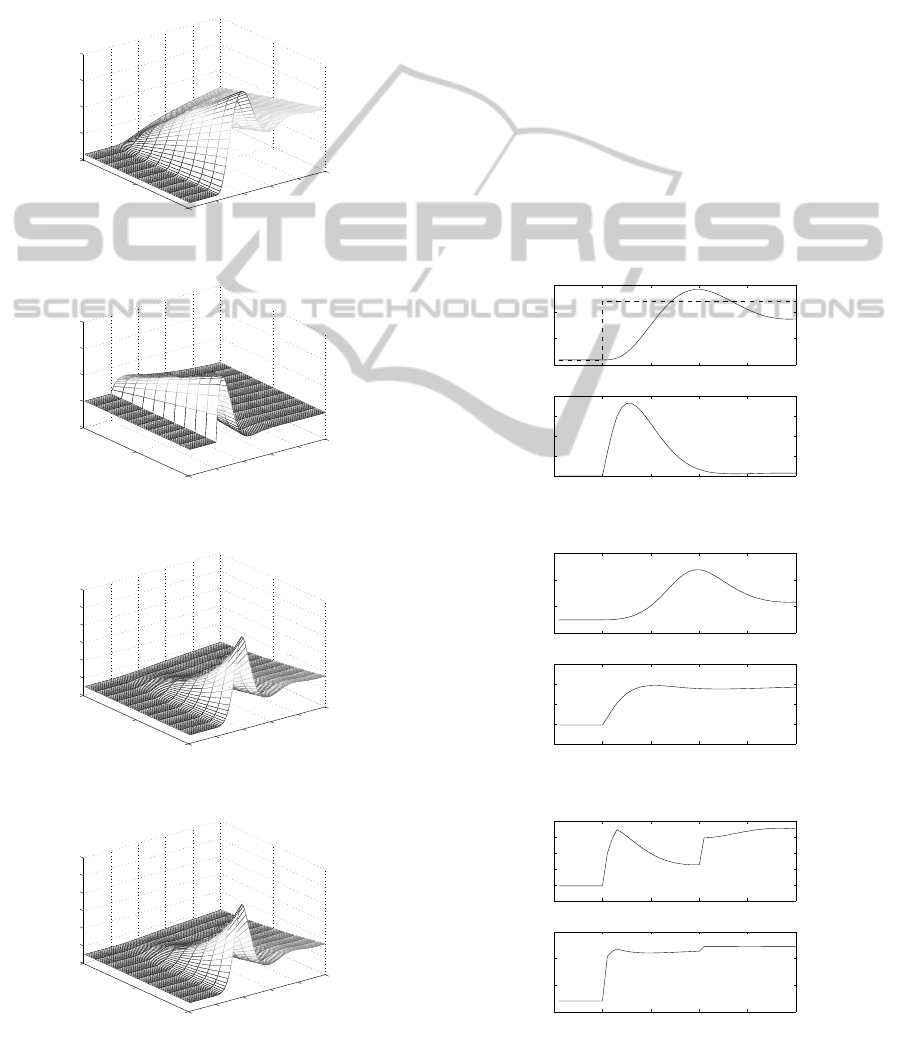
predictive control is working on discrete model. The
behaviour of constrained values can be however ob-
served through simulations. For the levitation systems
variables in function of time and α are presented in
figures 2 - 5.
As it can be seen every variable goes away from
constraints as α is increasing therefore the interpola-
tion method can be used.
0
1
2
3
4
5
0
0.5
1
0
0.005
0.01
0.015
0.02
time
alpha
x
1
Figure 2: ball position x
1
.
0
1
2
3
4
5
0
0.5
1
−0.1
0
0.1
0.2
0.3
time
alpha
x
2
Figure 3: ball velosity x
2
.
0
1
2
3
4
5
0
0.5
1
0
1
2
3
4
5
6
time
alpha
x
3
Figure 4: x
3
.
0
1
2
3
4
5
0
0.5
1
0
1
2
3
4
5
6
time
alpha
x
3
Figure 5: x
3
.
4 PROBLEM OF WEIGHTS IN
LINEAR QUADRATIC COST
As the objectiveof the control is to track the reference
trajectory and the constraints are fulfilled by the inter-
polation method it is possible to choose the weights
in LQ cost function and apply the algorithm. The
simulations presented in figures 6-8 are obtained with
weigth in quadratic cost function so chosen that for
every state variabe z
i
(values on diagolnal of q) and
control v
i
(the value R) equals 0.1 for both linear sys-
tems (5, 6). The model is augmented, so for the addi-
tional state variable which realize tracking the weight
equals 100. Unortunately obtained charts presents
very slow motion of the controlled ball.
Problem of choosing weights for the z state and v
control is more difficult than for model of known sig-
nals of physical meaning. Finding weights for vari-
ables x and u is easier as that signals usually repre-
0 0.5 1 1.5 2 2.5
0
0.005
0.01
0.015
time
x1
0 0.5 1 1.5 2 2.5
0
0.05
0.1
0.15
0.2
time
x2
Figure 6: ball position x
1
and velocity x
2
.
0 0.5 1 1.5 2 2.5
0
1
2
3
time
x3
0 0.5 1 1.5 2 2.5
0.45
0.5
0.55
0.6
0.65
time
x4
Figure 7: x
3
,x
4
.
0 0.5 1 1.5 2 2.5
0
0.2
0.4
0.6
0.8
1
time
u1
0 0.5 1 1.5 2 2.5
0.18
0.2
0.22
0.24
time
u2
Figure 8: control signals u
1
,u
2
.
InputandStateConstrainedNonlinearPredictiveControl-ApplicationtoaLevitationSystem
277

sent known physical variables. When one wants to
use that knowledgefor the linearizad model one meets
the problem of the nonlinear, multivariable functions
obtained from FBL (3, 4).
The way that can be used here is to confront the
cost function designed for the original nonlinear sys-
tem (for example for the purpose of linear quadratic
conttrol for system linearized in the point of work by
Jacobian linearization) with the function we need to
use for new linear system. In the example of levita-
tion system the first cost function has form:
J =
∞
∑
k=1
˜x
T
k
Q
x
˜x
k
+ ˜u
T
k
R
x
˜u
k
(22)
where
˜x(t) = x(t) − x
s
˜u(t) = u(t) − u
s
(23)
and x
s
,u
s
describe steady point for desired value of
y (the further value in vector w). The system should
be shifted (by using variables (23)) that ˜x
s
= 0, ˜u
s
=
0, but after feedback linearization the shift weights
sholud be considered in the weights values. If the Q
x
and R
x
are diagonal matrices then the cost function
for given k step is
F
x
= q
1
x
2
1
+ q
2
x
2
2
+ q
3
x
2
3
+ q
4
x
2
4
+ r
2
1
u
2
1
+ r
2
2
u
2
2
(24)
The function should be approximated with similar
function for linear system. In levitation example there
are two linear systems, therefore the two cost functons
can take form
F
z1
= [z
1
z
2
z
3
]Q
z1
z
1
z
2
z
3
+ v
2
1
R
z1
+ 2[z
1
z
2
z
3
]N
z1
v
1
(25)
F
z2
= z
2
4
Q
z2
+ v
2
2
R
z2
+ 2z
4
N
22
v
2
(26)
The cost functions for linear system should be close
to the function for nonlinear system, that is for the
levitation example
F
x
≈ F
z1
+ F
z2
. (27)
The method that can be used is the linear approxima-
tion in the point (y
s
,x
s
,u
s
) of two functions - diffeo-
morphism x(z) and control u(z,v) (obtained from (3,
4)) for every variable x
i
,v
j
. For the levitation system,
where
x
1
(z
1
,z
2
,z
3
,z
4
)
x
2
(z
1
,z
2
,z
3
,z
4
)
x
3
(z
1
,z
2
,z
3
,z
4
)
x
4
(z
1
,z
2
,z
3
,z
4
)
u
1
(z
1
,z
2
,z
3
,z
4
,v
1
,v
2
)
u
2
(z
1
,z
2
,z
3
,z
4
,v
1
,v
2
)
(28)
we can obtain linear approximation
x
i
≈
dx
i
dz
1
|
s
z
1
+
dx
i
dz
2
|
s
z
2
+
dx
i
dz
3
|
s
z
3
+
dx
i
dz
4
|
s
z
4
u
j
≈
du
j
dz
1
|
s
z
1
+ ... +
du
j
dz
4
|
s
z
4
+
du
j
dv
1
|
s
v
1
+
du
j
dv
2
|
s
v
2
(29)
where index s indicates, that in the obtained functions
variables from vectors z and v should be replaced by
values in desired point s (z
s
,v
s
). Variables x
i
and u
j
obtained in this way can be substitute into function
F
x
in order to obtain cost function with variables z
and v. It can happen (that was for the levitation sys-
tem) that for MIMO systems we can obtain fragments
of function that will not appear in the cost functions
for linear systems (F
z1
,F
z2
) (for example function of
(z
1
,v
2
)) and that fragments have to be simply omit-
ted. The weights for cost functions for LQ method
for linear systems are available from F
z
functions.
The procedure was proceeded for the levitation
example, where values of weights for nonlinear
variable were following: q
1
= 100,q
2
= 0.1,q
3
=
0.1,q
4
= 1,r
1
= 0.1,r
2
= 0.1. Simulation has been
prepared for the step of discretization T
s
= 0.05s and
the horizon h = 20. Obtained results are presented on
figures 9-11
0 0.5 1 1.5 2 2.5
0
0.005
0.01
0.015
time
x1
0 0.5 1 1.5 2 2.5
0
0.02
0.04
0.06
0.08
0.1
time
x2
Figure 9: ball position x
1
and velocity x
2
.
0 0.5 1 1.5 2 2.5
0
1
2
3
time
x3
0 0.5 1 1.5 2 2.5
0.45
0.5
0.55
0.6
0.65
time
x4
Figure 10: x
3
,x
4
.
5 CONCLUSIONS
Obtained results show that the method is valid for the
system, constraints are fulfilled (it is visible on charts
of x
3
and u
1
which are close to constraints; when sim-
ICINCO2014-11thInternationalConferenceonInformaticsinControl,AutomationandRobotics
278

0 0.5 1 1.5 2 2.5
0
0.2
0.4
0.6
0.8
time
u1
0 0.5 1 1.5 2 2.5
0.18
0.2
0.22
0.24
time
u2
Figure 11: control signals u
1
,u
2
.
ulations with too short horizon were implemented, the
constraints of the varaiables were violated). The min-
imized variable α, obtained in every step, was used
the same for both linear models (5, 6). Simulations
show how important is to choose proper weights val-
ues. For the first choice, when only diagonal values
for input and state was plased, performance of out-
put was very slow. Weights obtained by aproximation
and comparison to function with signals of physical
meaning improved the response.
As the weights are obtained through approxima-
tion, for hardly nonlinear models it can be convinient
to change that values for situations, when system
changes the working point. Nonetheless the algorithm
is based on exact linearization, therefore if propor-
tions of signals are similar to that of signals in ap-
proximation point the control law should be sufficient
for once calculated weights.
REFERENCES
Ahmad, A., Saad, Z., Osman, M., Isa, I., Sadimin, S., and
Abdullah, S. (2010). Control of magnetic levitation
system using fuzzy logic control. In Proc. of the Sec-
ond International Conference on Computational Intel-
ligence, Modelling and Simulation, pages 51–56, Bali.
Al-Muthairi, N. and Zribi, M. (2004). Sliding mode control
of a magnetic levitation system. Mathematical Prob-
lems in Engineering, (2004:2):93–107.
Bachle, T., Hentzelt, S., and Graichen, K. (2013). Nonlinear
model predictive control of a magnetic levitation sys-
tem. Control Engineering Practice, (21):1250–1258.
Dragos, C., Preitl, S., Precup, R., and Petriu, E.
(2012). Points of view on magnetic levitation sys-
tem laboratory-based control education. In Human-
Computer Systems Interaction, part II, pages 261–
275. Springer-Verlag, Berlin.
Isidori, A. (1995). Nonlinear Control Systems. Spinger-
Verlag, London.
Kang, C.-S., Park, J.-I., Park, M., and Baek, J. (2014).
Novel modeling and control strategies for a hvac
system including carbon dioxide control. Energies,
(7):3599–3617.
Khalil, H. (2002). Nonlinear Systems. Prentice Hall, New
Jersey.
mls2em (2009). Magnetic Levitation System. User’s Man-
ual. printed by InTeCo Ltd.
Poulsen, N., Kouvaritakis, B., and Cannon, M. (2001).
Nonlinear constrained predictive control applied to a
coupled-tanks apparatus. In IEE Proc. of Control The-
ory and Applications, volume 148, pages 17–24.
Yang, Z.-J. and Tateishi, M. (2001). Adaptive robust non-
linear control of a magnetic levitation system. Auto-
matica, (37:7):1125–1131.
Zietkiewicz, J. (2012). Constrained predictive control of
mimo system. application to a two link manipulator.
In Proc. of the 9th International Conference on In-
formatics in Control, Automation and Robotics, pages
293–298.
InputandStateConstrainedNonlinearPredictiveControl-ApplicationtoaLevitationSystem
279
