
Fuzzy Inference System to Analyze Ordinal Variables
The Case of Evaluating Teaching Activity
Michele Lalla
1
, Davide Ferrari
2
and Tommaso Pirotti
1
1
Marco Biagi Economics Department, University of Modena and Reggio Emilia, Modena, Italy
2
Department of Mathematics and Statistics, University of Melbourne, Melbourne, Australia
Keywords:
Ordinal Scales, Likert Scale, Student Evaluation, Fuzzification, Defuzzification.
Abstract:
The handling of ordinal variables presents many difficulties in both the measurements phase and the statistical
data analysis. Many efforts have been made to overcome them. An alternative approach to traditional methods
used to process ordinal data has been developed over the last two decades. It is based on a fuzzy inference
system and is presented, here, applied to the student evaluations of teaching data collected via Internet in
Modena, during the academic year 2009/10, by a questionnaire containing items with a four-point Likert
scale. The scores emerging from the proposed fuzzy inference system proved to be approximately comparable
to scores obtained through the practical, but questionable, procedure based on the average of the item value
labels. The fuzzification using a number of membership functions smaller than the number of modalities of
input variables yielded outputs that were closer to the average of the item value labels. The Center-of-Area
defuzzification method showed good performances and lower dispersion around the mean of the value labels.
1 INTRODUCTION
The purpose of the present paper is twofold. Firstly,
it briefly discusses the limits of some statistical in-
dices in representing synthetically ordinal variables,
which constitute the current or traditional procedures.
Secondly, the fuzzy approach, based on the FIS, is ap-
plied to data concerning student evaluations of teach-
ing activity (SETA). In fact, our data set contains pre-
vailingly ordinal information from an online survey
conducted by the University of Modena and Reggio
Emilia, for the Academic Year 2009/2010. The data
analysis was restricted to the evaluated courses in the
“Economics and International Management” degree
program of the Faculty of Economics. The fuzzy ap-
proach through FIS offers a clear advantage over tra-
ditional methods because it is highly flexible in han-
dling data and avoids the usual complications related
to measurement methodology. For example, the FIS
permits handling of both the four- or five-point Likert
scale and any other type of scale without theoretical
difficulties and great flexibility with a large variety of
solutions. A comparison between the results obtained
from current procedures and the proposed FIS will
be analyzed and described, illustrating the strengths
and weaknesses of both. A fuzzy inference model
may well be a new and different way to analyze or-
dinal variables and, specifically, student evaluations
of teaching activity.
2 ORDINAL SCALES
The objective of the measurements process is to ob-
tain information that is valid (i.e., it succeeds in evalu-
ating what it is intended to evaluate), reliable (i.e., the
results can be reproduced upon replication of the pro-
cedure, yielding identical or very similar values), and
precise (i.e., the multiples or submultiples of the unit
of measurement are contained by the available de-
vice). Given that it is not always possible to establish
or find the unit of measurement of social concepts,
preciseness remains a real difficulty of each inten-
sity concept’s evaluation, which is generally classified
on the basis of its nature and preciseness (Stevens,
1946), where the lowest level is based on discrimina-
tion (nominal) and the subsequent level is based on
an order relation (ordinal). The basic assumptions of
almost all ordinal scales are (1) the unidimensionality
of the surveyed concept, (2) the location of the con-
cept on a continuum, (3) the equidistance between the
modalities constituting the observable level of the in-
tensity of the concept.
Many techniques of scales have been developed
25
Lalla M., Ferrari D. and Pirotti T..
Fuzzy Inference System to Analyze Ordinal Variables - The Case of Evaluating Teaching Activity.
DOI: 10.5220/0005054400250036
In Proceedings of the International Conference on Fuzzy Computation Theory and Applications (FCTA-2014), pages 25-36
ISBN: 978-989-758-053-6
Copyright
c
2014 SCITEPRESS (Science and Technology Publications, Lda.)

since the 1920s to study attitudes and, to a lesser
extent, psychophysical and psychometric behavior
(White, 1926; Thurstone, 1927; Thurstone, 1928).
The ordinal scales most used in practice are ‘sum-
mated’ scales and one of the first successful proce-
dures to obtain an ordinal variable, whose values de-
note the intensity level of its denoted concept, was
proposed by Likert (1932) to measure attitudes and
opinions through statements. The intensity of each
statement was rated with graduated response keys
(modalities), originally seven: strongly agree, mildly
agree, agree, uncertain, disagree, mildly disagree, and
strongly disagree (seven-point Likert scale). Sub-
sequently, the alternatives containing “mildly” were
dropped, obtaining a five-point scale. The neutral
point presents a theoretical and empirical, unsolved
issue because many results do not give strong indica-
tions about the advisability of its presence/absence. It
is often eliminated (Schuman and Presser, 1996).
Let i be an index denoting the interviewed sub-
ject. Let j be an index denoting a concept, and k, a
statement or item about the j-th concept. The cor-
responding score, y
i jk
, belongs to {1, ... M} ⊂ N for
any statement favorable to the concept and it belongs
to {M, . . . 1} ⊂ N for any statement not favoring the
concept, where M is the number of points of the scale
(5 or 7) and N is the set of natural numbers. The j-
th concept is often measured through K
j
items (vari-
ables), forming a battery and semantically connected
to it. Each item, k, has a Likert scale with M
k
modali-
ties, in general, but often M
k
is the same for all items.
The answer of the i-th respondent gives an outcome
x
i jk
in (1, 2, 3, 4 [, 5, 6, 7]). The sum (x
i j
) or the mean
( ¯x
i j
) of the K
j
natural numbers yields a measure of the
intensity of the j-th concept
(a) x
i j
=
∑
K
j
k=1
x
i jk
or
(b) ¯x
i j
= (1/K
j
)
∑
K
j
k=1
x
i jk
(1)
The sum is sometimes rescaled to one (or ten), y
i j
,
through the expression y
i j
= (x
i j
− x
min j
)/(x
max j
−
x
min j
), for the i-th individual and the j-th concept,
where the x
min j
and x
max j
are, respectively, the max-
imum and the minimum of x
i j
in the data set. But, this
calculus is not admissible as the average and the sum
because the device generates only ordinal data.
The semantic differential scale is another ordinal
scale (Osgood, 1952; Osgood et al., 1957) and in its
usual or standard format, it consists of a set of seven
categories, but they may vary in number, associated
with bipolar adjectives or phrases. For each bipolar
item, the respondent indicates the extent to which one
descriptor represents the concept under examination.
The semantic differential scale is aimed at measur-
ing direction (with the choice of one of two terms,
such as ‘useful’ or ‘useless’) and extent/amount (by
selection of one of the provided categories express-
ing the intensity of the choice). The volume of mea-
surements is generally high and the interpretation of
the results of word scales is theoretically based on
three factors (‘evaluation’, ‘potency’, and ‘activity’),
which involves fairly complex analyses requiring ex-
pensive data-processing procedures. Therefore, the
objectives of these theoretical scales may necessarily
involve long-term research, limiting their applicabil-
ity or often subjecting them to simplified analysis and
thus reducing some of their potential (Yu et al., 2003).
The Stapel scale is a ten-point non-verbal rating
scale, ranging from +5 to -5 without a zero point and
measuring direction and intensity simultaneously. It
has been stated that “it cannot be assumed that the in-
tervals are equal or that ratings are additive” (Crespi,
1961), but the Stapel scale is used under the same as-
sumptions as the Likert scale. With respect to seman-
tic differential, the Stapel scale presents each adjec-
tive or phrase separately and the points are identified
by number. The use of a ten-point scale is more intu-
itive and common than the seven-point scale.
The self-anchoring scale is another type of ordinal
scale and, in its usual or standard format, it consists of
a graphic, non-verbal scale, such as the ten-point lad-
der scale (Kilpatrick and Cantril, 1960; Cantril and
Free, 1962), where respondents are asked to define
their own end points (anchors). The best is at the top,
if the ladder is in vertical position (case 1), or at the
right, if the ladder is in horizontal position (case 2).
The worst is at bottom in the first case and on the
left in the second case. It is a direct outgrowth of the
transactional theory of human behavior in which the
‘reality world’ of each of us is always to some extent
unique, the outcomes of our perceptions being con-
ceived as ongoing extrapolations of the past related to
sensory stimulation. The scale may solve some prob-
lems and biases typical of category scales, but it is
often used as fixed anchoring rating scale, where the
anchor of the scale is already defined, assuming, im-
plicitly, the existence of an objective reality.
The feeling thermometer scale was developed by
Clausen for social groups and was first used in the
American National Election Survey (ANES), 1964. It
was later modified by Weisberg and Rusk (1970). Its
format is like a segment of a 0-to-100-degree temper-
ature scale, which reports some specific values. In the
evaluation of political candidates, it was “a card list-
ing nine temperatures throughout the scale range and
their corresponding verbal meanings as to intensity
of ‘hot’ or ‘cold’ feelings was handed to the respon-
dent” (Weisberg and Rusk, 1970).
Roughly speaking, the Stapel, self-anchoring, and
FCTA2014-InternationalConferenceonFuzzyComputationTheoryandApplications
26

feeling thermometer scales are structurally similar to
thermometer scales that have a long history, although
they are often ascribed to Crespi (1945a, 1945b) as
cited, for example, by Bernberg (1952). However, the
thermometer scales used in social sciences do not pro-
vide values on interval scales, as does a thermometer
used to measure temperatures.
Among other ordinal scales, the Guttman scale is
a method of discovering and using the empirical in-
tensity structure among a set of given indicators of
a concept. The Bogardus social distance scale mea-
sures the degree to which a person would be willing
to associate with a given class of people - such as an
ethnic minority (Babbie, 2010). The Juster scale is an
11-point scale, like a decimal scale, used for predict-
ing the purchase of consumer durables and for each
question asking people to assign probabilities to the
likelihood of their adopting the described behavior on
that question (Juster, 1960; Juster, 1966).
There is no rationale in the practice of handling
the figures assigned to the modalities of an ordinal
scale as real numbers, also under the assumption of
equidistance between the categories. It is possible to
envisage the selection of a modality as an output of a
normal variable underlying a random discriminatory
process, which could justify the use of equations (1)
exploiting the properties of the normal random vari-
ables. However, if the modalities are subordinate only
to a relation order, the use of the sum and the mean re-
mains problematic.
3 STUDENT EVALUATION OF
TEACHING ACTIVITY
The students’ opinions about teaching activity rose to
the attention of the academic administrations in the
1920s and some US universities such as Harvard, the
University of Washington and Texas, Purdue Univer-
sity, and other institutions, introduced student eval-
uations as a standard practice (Marsh, 1987). Since
then, many aspects have been investigated, such as the
reliability, validity, unbiasedness, efficiency, and effi-
cacy of SETA. Moreover, many more universities in
the US and other countries have introduced the prac-
tice of evaluating teachers and course organization.
3.1 The Course-evaluation
Questionnaire
In Italy, the evaluation of university teaching activ-
ities and research is regulated by Law no. 370 (of
19/10/1999, Official Gazette, General Series, no. 252
of 26/10/1999), which also does not allow adminis-
trations failing to comply with it to apply for certain
grants. The same law established the National Com-
mittee for University System Evaluation (Comitato
Nazionale di Valutazione del Sistema Universitario,
CNVSU), replacing the Observatory for University
System Evaluation. A research group of the CNVSU
(2002) proposed a standard course evaluation ques-
tionnaire with a minimum set (battery) of fifteen items
for all universities. Each item includes the follow-
ing four-point Likert scale: 1 Definitely no, 2 No
rather than yes, 3 Yes rather than no, 4 Definitely
yes (CNVSU scale). A traditional item-by-item anal-
ysis was generally carried out, using means and vari-
ances of numerical values obtained by translating
the categories (or labels) into a ten-point scale as
follows: 1 =2, 2 =5, 3 =7, 4 =10, hereinafter re-
ferred to as numeric values of labels. One could argue
that the absence of a mid value on this ordinal scale
could violate the linearity assumption and the mean
and variance analysis cannot validly be used. More-
over, the meaning of the labels might not be clear to
all students. Hence, the intensities, or degree of cer-
tainty, associated with these labels often correspond
to a high level of vagueness; investigations of these
topics are reported elsewhere (Lalla et al., 2004).
In the Academic Year 2004/2005, the Committee
for Technical Evaluation of the University of Mod-
ena and Reggio Emilia adopted the questionnaire pro-
posed by CNVSU (2002) and in the Academic Year
2005/2006, it introduced the online survey for SETA
(Lalla and Ferrari, 2011). Some minor changes in-
volved a slight modification of the wording of some
items (to make their meaning clearer) and the order
of the items (to reduce the halo effect). The overall
questionnaire contained seven sections, but Sections
I (personnel data, containing information about the
course, teacher, and some student characteristics) and
VII (remarks and suggestions, listing nine items with
dichotomous choices) are not presented here. Sec-
tions from II to VI represent the core of the question-
naire and contain a 15-item battery with the four-point
Likert scale to achieve the standard evaluation (Table
1). The current procedure generates the evaluation
of a single item or domain, which is performed us-
ing the traditional procedure of averaging (over the
sample) the numerical labels or the assigned values
corresponding to a ten-point scale
¯x
jk
= (1/n)
∑
n
i=1
x
i jk
(2)
Although the items included in a domain are assumed
to have the same importance in the arithmetic mean,
one could argue that certain variables indicating the
efficiency of the course are more important than oth-
FuzzyInferenceSystemtoAnalyzeOrdinalVariables-TheCaseofEvaluatingTeachingActivity
27

Table 1: Questionnaire items with median (md), mean ( ¯x), standard deviation (σ), and number of valid cases (n) for the
“Economics and International Management” degree program: Academic Year 2009/2010.
Questionnaire items – Total n=4537 Acronym md ¯x σ n
S. II Organization of this course
I01: Adequacy of the Work Load required by the course awl 7 6.5 2.2 4500
I02: Adequacy of the Teaching Materials atm 7 7.3 2.0 4472
I03: Usefulness of Supplementary Teaching Activity (STA) usta 7 7.2 2.1 2503
I04: Clarity of the Forms and rules of the Exams cfe 7 7.3 2.2 4429
S. III Elements concerning the teacher
I05: Reliability of the Official Schedule of Lectures rosl 7 8.0 2.1 4460
I06: Teacher Availability for Explanations tae 7 7.8 1.9 4442
I07: Motivation and Interest generated by Teacher mit 7 7.2 2.2 4449
I08: Clarity and Preciseness of the Teachers Presentations cptp 7 7.4 2.1 4427
S. IV Lecture room and resource room
I09: Adequacy of the Lecture Room alr 7 7.2 2.1 4444
I10: Adequacy of the Room and Equipment for STA aresta 7 7.2 2.1 2475
S. V Background-interest-satisfaction
I11: Sufficiency of Background Knowledge sbk 7 7.0 2.0 4442
I12: Level of Interest in the Subject matter lis 7 7.4 2.1 4444
I13: Level of Overall Satisfaction with the course los 7 7.1 2.1 4418
S. VI Organization of all courses in the degree program
I14: Adequacy of the Total Work Load of current courses atwl 7 6.0 2.2 4452
I15: Feasibility of the Total Organization (lect. & exams) fto 7 6.1 2.2 4445
ers. To take into account these differences, one ap-
proach is to use a weighted average. Still, the choice
of the weights is a controversial point due its arbitrari-
ness. Moreover, it could be noted that the median,
which is the correct statistical index for ordinal vari-
ables, is less informative of the mean in summarizing
the distribution of the answers, as is evident, but ques-
tionable, from the data reported in Table 1.
4 FUZZY INFERENCE SYSTEMS
The structure and functioning of a FIS follow defined
hierarchical steps (Dubois and Prade, 2000).
4.1 The FIS for Teaching Evaluation
Issue identification (i) involves a stepwise proce-
dure that could be carried out through a top-down
or bottom-up strategy. In the first case, it is simi-
lar to a scientific inquiry. It starts from the output
variables and attempts to identify macro-indicators -
possibly including multiple input variables - that can
adequately explain the output. The macro-indicators
are subsequently broken down into smaller indica-
tors that include fewer variables. The stepwise pro-
cess continues until the single input variables are iso-
lated. The final product is a modular tree-patterned
system, where several fuzzy modules are interlinked.
In the bottom-up strategy, the input variables are al-
ready available, as is the case examined here, and
the goal consists in subsequently aggregating them.
Each aggregation generates a fuzzy module. The var-
ious modules are interlinked with each other. The
final emerging arrangement is like a tree-patterned
structure generating a single (or multiple) output(s).
An example of the latter is the model considered for
SETA, which includes the 15-item battery and item
aggregation, from input to final output (Figure 1). The
variables enter the system at different levels of impor-
tance, which heavily affects the final output. Roughly
speaking, the approach corresponds to a weighted av-
erage, where the weights are unknown and higher
for variables entering the last steps. The aggregat-
ing function is generally unknown and not necessar-
ily linear, as in a weighted average. In the FIS, each
aggregation of variables gives an intermediate solu-
tion, which is a fuzzy set variable and it does not
have necessarily a particular meaning attached to it.
Sometimes, however, the intermediate variables do
have a useful meaning. For example, the aggrega-
tion of AWL and ATM generates the new intermediate
fuzzy variable OMW (Organization of Materials and
Workload), while the aggregation of USTA and CFE
generates the new intermediate fuzzy variable OEE
(Organization of Exercises and Exams). In a subse-
quent step, the aggregation of OMW and OEE gener-
ates OC (Organization of the Course). The merging
FCTA2014-InternationalConferenceonFuzzyComputationTheoryandApplications
28

of fuzzy modules will continue up to the aggregation
of OC with TTC (Total Teaching Capability), obtain-
ing SET (Student Evaluation of Teacher). To account
for student satisfaction, SET is aggregated with LOS,
the level of overall satisfaction of students, obtaining
SETS (Student Evaluation of Teacher plus Satisfac-
tion). The adopted level of inclusion involves a strong
influence of satisfaction on SETS, while a mitigation
of its effect could be obtained, firstly, by combining
TTC or OC with LOS and, secondly, by merging the
result with OC or TTC, as reaffirmed in the comments
on the results reported below.
The fuzzification of input, (ii), involves the speci-
fications concerning the shapes and the number of the
membership functions (mf) for the input variables. A
membership function defines the extent to which each
value of a numerical variable belongs to some speci-
fied categorical labels. In the following, we briefly
describe the most popular approaches used to deter-
mine their shapes (Smithson, 1988). (1) The survey
approach determines the shapes of the membership
functions based on information from a specifically de-
signed sample. For this purpose, a common choice is
to use empirical sampling distributions from the par-
ticular collected data concerning the intensity of the
value labels. (2) The comparative judgment approach
defines the functions through a comparison of stimuli
and some given features or prototypes. (3) The expert
scaling approach characterizes the function in accor-
dance with the subjective experience of an expert. (4)
The formalistic approach selects functions with spe-
cific mathematical properties. (5) Machine-learning
builds up the functions from a set of past data (train-
ing and testing data set) and transfers the same struc-
ture to the present and future.
The aim of SETA is to collect student opinions
about the teachers and the course organization. There-
fore, approach (1) is preferable because it allows for
direct measurement of the meaning that students at-
tribute to the linguistic options/categories on the 15-
item battery. In particular, each sampled student
should assign scores for each category of the CN-
VSU scale denoted by a label, for each of the 15-
items. This permits construction of frequency poly-
gons, which give approximate representations of the
vagueness level of the category choices. The poly-
gons translate the decimal value of each category into
a corresponding membership level for the popula-
tion. This strategy could be costly, as all surveys are
costly, and it presents some degree of difficulty due to
the nuisance, laboriousness, and repetitiveness of the
task. Actually, each student should assign scores for
15 × 4 elements. In fact, the evaluation of the same
four response options is repeated fifteen times, the
Figure 1: The structure of the Fuzzy Inference System for
student evaluation of teaching activity.
number of items on the CNVSU questionnaire. As
a consequence, the procedure requires a large sample
of students and a well-designed strategy for data col-
lection. Moreover, given that the empirical frequency
polygons are somewhat irregular, their final shapes
could be determined taking into account method (2)
in order to smooth and simplify the forms of the fre-
quency polygons with respect to both the theoreti-
cal constraints and the aims of the FIS. In general,
the frequency polygons are well fitted by probability
distribution, such as normal, gamma, and beta, but
they are also well approximated by triangular (a,α,β)
or trapezoidal (a, b, α, β) shapes centered about the
means of the score distributions for each modality.
With respect to other strategies, approach (3) is in-
adequate for teaching evaluation because the experts’
opinions might not match those of students. Ap-
proach (4) does not fit our purposes simply because
a priori mathematical properties do not necessarily fit
the reality of our data (although in many situations
they produce smoothed and tractable functions). Fi-
nally, approach (5) also appears to be inappropriate
because past data on the numerical values for the scale
categories are not available and are probably not time-
invariant.
The membership functions of some input vari-
ables for the FIS, in Figure 1, could be deduced from
the survey carried out in October 2000, where the
modalities of eight items were evaluated by students
FuzzyInferenceSystemtoAnalyzeOrdinalVariables-TheCaseofEvaluatingTeachingActivity
29

using a decimal scale (Lalla et al., 2004; Lalla and
Facchinetti, 2004). Only eight items (seven of them
about the teacher) were available out of fifteen, but
the scores refer to different formats and ten years
have already passed. Therefore, a simple fuzzifica-
tion was adopted, assuming as membership functions
trapezoidal or triangular shapes and considering the
symmetry about some specific values in the decimal
scale range or the value labels of the modalities (Grze-
gorzewski and Mr
´
owka, 2005; Grzegorzewski and
Mr
´
owka, 2007; Grzegorzewski, 2008; Yeh, 2009). In
fact, the relative frequency polygons could be well ap-
proximated by triangular shapes centered about the
means of the score distributions for each category.
The triangularization of the membership functions of
the input variable is a common practice, but it in-
volves a right-angled triangle for the first and the last
modality, i.e., the first and the last triangle. Hence, the
following types of fuzzification were considered. The
first type used three membership functions (mf3); this
number is lower then the number of modalities (4) to
allow the activation of two membership functions for
the internal modalities. The triangular fuzzy numbers
(a,α,β) had peaks a = (2, 6,10) and the left width
α was equal to the right width β, i.e., α = β = 4, as
in Figure 2 generated by “fuzzyTECH” (N.N., 2007).
The domain of the membership functions ranged from
2 to 10 and the response of the FIS was restricted to
the interval [2, 10] because the traditional means of the
numerical values attributed to the CNVSU scale cate-
gories, D = {2,5,7,10}, clearly ranged from 2 to 10.
Note that there are also many other possible choices
and modifications of the shapes for improvement of
the performances of the FIS.
There is also the possibility of using trapezoidal
fuzzy numbers. For example, the first membership
function is a trapezoidal fuzzy number, (a,b,α,β),
with peak (a = 2,b = 3), left width α = 0 and right
width β = 3. The second function is triangular shaped
(a,α,β), with peaks a = 6, left width α = 3, and right
width β = 3. The third, which is also the last, would
be a trapezoidal fuzzy number again (a,b,α,β), with
peak (a = 9,b = 10), left width α = 3 and right width
β = 0. The structure with two trapezoids, at the ex-
tremes of the decimal scale, could emphasize the FIS
scores towards the upper and lower bounds of the sup-
port (Lalla et al., 2004) in some defuzzification meth-
ods. However, it was not used here.
The second type used four membership functions
(mf4). This number was equal to the number of
modalities, implying that, in the absence of any other
information out of the symmetry and the range of nu-
meric values of the CNVSU scale categories, the tri-
angular fuzzy numbers (a,α,β) had peaks coinciding
Figure 2: Fuzzification of an input variable using three tri-
angles as membership functions (mf).
with the numeric values a = (2, 4.
¯
6,7.
¯
3,10) and the
left width α was equal to the right width β, i.e., α =
β = 2.
¯
6, as generated by “fuzzyTECH” (N.N., 2007)
in Figure 3. In this case, the most natural pattern may
be a fuzzification with peaks in a = (2,5,7,10) and
different values of the left width α and the right width
β. In other terms, the membership function associ-
ated with a fixed modality is represented by a triangle
with the peak centered on its value on the scale and
the amplitude ranging from the first lower to the first
upper modality. Therefore, it tends to confine the re-
sults to the selected modalities and the FIS does not
work completely, but only through the rule-blocks,
thus partially losing its nature.
In formal terms, the indices j and k of x
i jk
are sum-
marized in a single index l to simplify the formalism.
Therefore, let x
il
, l = 1,...,L, be the input variables
(L = 15 in the examined case) provided by the i−th
student with range U
l
and let y be the output variable
with range V . Let M(l) be the number of categories
of x
l
. Generally, such a number could change from
one variable to another, but in this case, M(l) = 4
(the number of CNVSU scale options/categories) for
all l = 1,...,L. Therefore, in general, an effective
fuzzification of input requires a number of member-
ship functions greater than one and less than M(l).
Moreover, each category of x
l
is described by a fuzzy
number, A
l
j(l)
, ∀ j(l) ∈ [1, . . . , M(l)], and the set A
l
=
{A
l
1
,...,A
l
M(l)
} denotes the fuzzy input x
l
, while the
fuzzy output of y is defined by B = {B
1
,...,B
M(y)
}
where M(y) denotes the number of membership func-
tions (or categories or modalities) for y. Each set has
a membership function:
µ
A
l
j(l)
(x) : U
l
→ [0,1] µ
B
m
(x) : V → [0,1] (3)
The construction of rule-blocks, (iii), concerns the
relationships between the input linguistic variables
and output linguistic variables. It involves a multi-
criteria situation, described by a number of rules like:
R
s
: IF [x
1
is A
1
j(1)
⊗...⊗x
L
is A
L
j(L)
] THEN (y is B
m
) (4)
FCTA2014-InternationalConferenceonFuzzyComputationTheoryandApplications
30

Figure 3: Fuzzification of an input variable using four trian-
gles as membership functions (mf).
for all combinations of j(l) ∈ [1, . . .,M(l)] and m ∈
[1,... , M(y)]. The left-hand side of THEN is the an-
tecedent (premise) and the right-hand side is the con-
sequent (conclusion). The symbol ⊗ (otimes) denotes
an aggregation operator, one of several t-norms (if the
aggregation is an AND operation) or t-conorms (if the
aggregation is an OR operation). The aggregation op-
erator, AND, that was chosen, produces a numerical
value α
s,m
∈ [0, 1] and the latter represents the exe-
cution of the antecedent in rule R
s
. The α
s,m
num-
ber should be applied to the consequent membership
function of B
m
, in order to calculate the output of each
rule. The AND aggregation operator was used once
again, but in a slightly different context: ⊗ works on
a number and the membership function of a fuzzy set
B
m
, whereas in the case of the R
s
rule, it is applied on
two numbers (Von Altrock, 1997). An example of the
rule-block is presented for the fuzzy module OMW
(organization of material and workload) aggregating
AWL and ATM (Figure 1) and using the numeric val-
ues instead of labels, for the sake of brevity (three
membership functions):
• IF AWL is mf1 and ATM is mf1, THEN OMW is mf1
• IF AWL is mf1 and ATM is mf2, THEN OMW is mf2
• IF AWL is mf1 and ATM is mf3, THEN OMW is mf3
• IF AWL is mf2 and ATM is mf1, THEN OMW is mf2
• IF AWL is mf2 and ATM is mf2, THEN OMW is mf3
• IF AWL is mf2 and ATM is mf3, THEN OMW is mf4
• IF AWL is mf3 and ATM is mf1, THEN OMW is mf3
• IF AWL is mf3 and ATM is mf2, THEN OMW is mf4
• IF AWL is mf3 and ATM is mf3, THEN OMW is mf5.
It is possible to generate these rules automatically
through an algorithm, but an expert may express them
in a form that more closely fits the reality.
The aggregation of rule-blocks, (iv), is the step
of the evidential reasoning incorporating the pro-
cess of unification of the outputs of all the rules
in a single output Y. For every rule (R
s
) involved
in the numerical inputs, µ(α
s,m
⊗ B
m
), a different
output is obtained. These membership functions of
fuzzy sets have to be aggregated by an OR opera-
tion using a t-conorm. The most frequently used are
the max conorm, the probabilistic conorm, and the
Lukasiewicz conorm usually known as the bounded
sum. Now, the response of a module is ready, but it
is still in a fuzzy form. If the module needs to be ag-
gregated with other modules, the aggregation process
continues. Otherwise, it is an output module, even if
it is not the last output module, implying that it needs
to be changed back into a number to provide an easy
understanding of the system response.
Defuzzification of output, (v), is the process that
maps the output fuzzy set µ
B
(y) into a crisp value,
y
i j
, for the i-th student and j-th fuzzy module or con-
cept; i.e., it concentrates the vagueness expressed by
the polygon resulting from the activated output mem-
bership functions into a single summary figure that
best describes the central location of an entire poly-
gon. There is no universal technique to perform de-
fuzzification, i.e., to summarize this output polygon
by a number, as each algorithm exhibits suitable prop-
erties for particular classes of applications (Van Leek-
wijck and Kerre, 1999). The selection of a proper
method requires an understanding of the process that
underlies the mechanism generating the output and
the meaning of the different possible responses on
the basis of two criteria: the “best compromise” and
the “most plausible result”. Moreover, in an ordi-
nal output, with modalities described by linguistic ex-
pressions, their corresponding real values are always
given by the membership definitions, where the un-
derstanding of their meaning plays a key role.
For the first criterion, one of the most popu-
lar methods is the Center-of-Maxima (CoM), which
yields the best compromise between the activated
rules (Von Altrock, 1997). Given that more than
one output membership function could be activated
or evaluated as a possible response for the i-th student
and j-th fuzzy module or concept, let M
F;i j
be the
number of output- activated membership functions.
Let y
i jm
be the abscissa of the maximum in the m-
th activated output membership function. If the latter
has a maximizing interval, y
i jm
will be the median of
this interval. The final output crisp value, y
CoM;i j
, is
given by an average of membership maxima weighted
by their corresponding level of activation, µ
out;k
,
y
CoM; i j
=
∑
M
F; i j
m=1
µ
out; m
y
i jm
∑
M
F; i j
m=1
µ
out; m
(5)
The method of the center of area/gravity (CoA/G) was
excluded because it cannot reach the extremes of the
range [2,10] without fuzzification of input and output
on an interval wider than [2,10], which may seem un-
natural. In fact, it would have been possible to pick a
more suitable fuzzification of the input, but, in gen-
eral, FIS might produce an output greater than the
maximum or lower than the minimum of the scale.
FuzzyInferenceSystemtoAnalyzeOrdinalVariables-TheCaseofEvaluatingTeachingActivity
31

For the second criterion, the Mean-of-Maxima
(MoM) method yields the most plausible result, de-
termining the system output only for the membership
function with the highest resulting degree of the sup-
port. If the maximum is not unique, i.e., it is a maxi-
mizing interval, the mean of the latter is the response
y
MmM; i j
= max
l<=m<=M
F; i j
(y
i jm
) (6)
This approach selects the typical value of the terms
that is most valid, instead of balancing out the differ-
ent inference results (Von Altrock, 1997). Therefore,
it is often used in pattern recognition and classifica-
tion applications, as in the case of an ordinal output
whose modalities are described by linguistic expres-
sions, because the most plausible solution is more ap-
propriate instead of the mean.
In addition, the sensitivity analysis, (vi), is a pos-
sible sixth step that may be carried out to adapt the
FIS to the real situations that it would represent. The
FIS is handled as a parametric model, relating input
variables to membership functions, to fuzzy rules, to
hedges operations, to aggregations, and so on.
5 EMPIRICAL RESULTS
The academic year 2009/2010 was fixed as the ref-
erence date and the degree program in Economics
and International Management was selected out of
three undergraduate degree programs of the Faculty
of Economics. Some restrictions were imposed to the
overall dataset of 4537 (evaluating) students (Table
1), even if some analyses suggesting such restrictions
are not reported here for the sake of brevity. The
course-teacher is a unique combination because the
same teacher may teach more than one course and in
the same course there may be more than one teacher.
Five courses had less than twenty evaluating students
and these courses were thus eliminated, leading to a
reduction of 55 cases.
The complete elimination of nonresponses is not
the ideal strategy as it is too costly, it implies a loss of
cases and biases the estimates because nonresponses
do not randomly occur. However, considering the na-
ture of SETA data, if all items concerning the teacher
(I01-I08, I13), or all items concerning the organiza-
tion (I09, I10, I14, I15), were missing in a case, that
case was dropped. Fifty-four cases were lost through
this control, prevailingly owing to missing values for
all items referring to the teacher. Background knowl-
edge (I11) was used to replace the level of interest in
the subject matter (I12) when the latter was missing
and vice versa; if both were missing, they were re-
placed with the mean of teacher items. Therefore,
they did not involve a loss of cases. If in the 15-
item battery there were more than 8 (threshold) miss-
ing values in a single case (student), that case was
dropped: 17 cases crossed the threshold. In the end, a
total of 4411 cases were used.
The remaining missing values were replaced on
the basis of the available data for each single case
and considering that an evaluating student expressed
an opinion about three main areas (Figure 1): Stu-
dent evaluation of teacher plus satisfaction (SETS),
student’s perception of own position (SPOP), and to-
tal evaluation of facilities and organization (TEFO).
For each student, i, the k-th item belonging to a cer-
tain area with a missing value was replaced with the
mean of the values for the non-missing items of the
same area provided by the same student and not by the
mean of the k-th item for the total sample, as is usual.
For example, let I02(i), which belongs to SETS, be
missing; it was then replaced by the mean of [I01(i),
I03(i), I04(i), I05(i), I06(i), I07(i), I08(i), I13(i)]. Let
I02(i) and I13(i) be missing; they were then replaced
by the mean of [I01(i), I03(i), I04(i), I05(i), I06(i),
I07(i), I08(i)]. The rationale of this procedure relies
on the core of the evaluation process, which is the
evaluator. Therefore, the value used in the substitu-
tion is anchored to his/her average level of judgment
and not to the average level of the total sample. The
number of replaced values varied from one item to
another, ranging from 0.1% to 1%, except for sup-
plementary teaching activity (I03) and adequacy of
the room and equipment for the supplementary teach-
ing activity (I10), as those activities were not always
present in a course, implying an obvious high rate of
absence of evaluations for that particular item.
5.1 Student Evaluations of Teachers
The analysis has been prevailingly restricted to the
subsystems concerning the student evaluations of
teachers (SET) and SET plus satisfaction (SETS), as
indicated in Figure 1, for the sake of brevity and ow-
ing to the possibility to simulate the input data, as in-
dicated below. The traditional evaluation of teachers
currently in use, from the i-th student, is given by the
mean of the value labels assigned to the four modali-
ties of each item:
(a) ¯x
set;i
= (x
01;i
+ ··· + x
08;i
)/8
(b) ¯x
sets;i
= (x
01;i
+ ··· + x
08;i
+ x
13;i
)/9 (7)
The output of a FIS, x
FIS; i
, depends on the de-
cisions taken at each step. Specifically, the CoM
method used in the defuzzification step, with 3 or 4
membership functions in the fuzzification of input,
CoM3 or CoM4, generated x
CoM3; i
and x
CoM4; i
, re-
spectively. Analogously, the MoM method used in
FCTA2014-InternationalConferenceonFuzzyComputationTheoryandApplications
32

the defuzzification step, with 3 or 4 membership func-
tions in the fuzzification of input, MoM3 or MoM4,
generated x
MoM3; i
and x
MoM4; i
, respectively.
The rank of course-teachers may be a useful tool
to identify critical situations, where to offer sugges-
tions to the teacher or to urge him/her to improve
his/her behavior, the scope of the program, the teach-
ing materials, and so on. For this purpose, an item-
by item analysis could help persons in charge of aca-
demic organization and/or teachers, but here the re-
sults are limited only to the overall evaluation of the
teacher. The first and last positions of the rank are
reported in Table 2. The mean of the value labels,
¯x
set
, was lower than the fuzzy outputs ( ¯x
CoM3
, ¯x
MoM3
,
¯x
CoM4
, ¯x
MoM4
). The CoM3 fuzzy evaluations were
higher than those obtained by the mean of the value
labels and the mean of differences was 0.55, with the
lowest standard deviation (sd) being 0.45. The MoM3
provided crisp values that were close to CoM3 evalu-
ations and closer to ¯x
set; i
. In fact, the mean difference
was 0.41 (sd=0.63). Assuming the mean of the value
labels as a benchmark, ¯x
set; i
, the differences proved to
be slightly higher than 5%, on the average. Moreover,
the fuzzification with 4 membership functions did not
work as well as the fuzzification with 3 membership
functions because the outputs generally showed an in-
crease in the differences with respect to ¯x
set; i
. Op-
posite results were obtained by CoM4 and MoM4,
i.e., the CoM4 fuzzy evaluations yielded crisp values
closer to ¯x
set; i
than those yielded by MoM4. In fact,
the means of the differences with respect to ¯x
set; i
were
0.49 (sd=0.64) and 0.86 (sd=0.99), respectively.
The fuzzy outputs, x
FIS; i
, and the mean of the
value labels, x
set; i
, for the i-th student measure the
performance of a teacher. Therefore, they should
be correlated and an analysis of the relationships be-
tween the different fuzzy outputs and ¯x
set; i
clarifies
the structure of some differences. The scatter-plots of
fuzzy evaluations of teachers (SET) against the mean
of the corresponding value labels are reported in Fig-
ure 4. The estimates of the linear regression param-
eters between the four dependent variables (x
CoM3; i
,
x
MoM3; i
, x
CoM4; i
, x
MoM4; i
) on ¯x
set; i
, as the independent
variable, are reported in Table 3. If x
FIS; i
and ¯x
set; i
are
the same, one can expect a slope (β
1
) of the regression
line equal to 1 and an intercept (β
0
) equal to 0. The
correlative t-tests showed that these hypotheses were
always rejected, but the relationships were always ap-
proximately linear. The assumption of constant vari-
ance was refused in all models and the coefficients of
determination were sufficiently high.
The result closer to the hypotheses, notwith-
standing their rejection, was given by CoM3, which
showed residuals with the lowest standard deviation
SET
CoM3
SET
MoM3
SET
CoM4
SET
MoM4
Figure 4: Output fuzzy variables against the mean of the
value labels.
[sd(res-CoM3)=0.45] and a bimodal shape. MoM3
provided residuals with a notable dispersion [sd(res-
MoM3)=0.63] and a bell-shaped distribution. Cor-
respondence between the mean of the value labels
and the fuzzy outputs by CoM4 and MoM4 was
poorer in terms of the slope and the shapes or dis-
persion of residuals: sd(res-CoM4)=0.58 and sd(res-
MoM4)=0.95. For the sake of brevity the figures
were not reported here. Therefore, as expected, FIS
works better when the number of membership func-
tions for each x
il
input variable is lower than its num-
ber of modalities, M(l). Reasonably, the number of
input membership functions for the x
il
input variable
should range from 2 to [M(l) − 1]. Moreover, for
fuzzy output ordinal variables, MoM is more suitable
than CoM because it chooses the most plausible result
among the possible M
F; i j
results.
5.2 Simulated Data: All Possible Inputs
The mean of the value labels and of the FIS outputs
yielded measurements that often did not coincide, as
noted regarding the results in Tables 2-3. The differ-
ences between the mean of the FIS outputs and the
mean of the value labels were statistically different
from zero for both the total sample and the single
course teacher. However, the surveyed data did not
present all the possible combinations of input values
because many evaluation patterns were frequently re-
peated and others were never expressed by students.
Therefore, the previous analysis was repeated using
a simulated dataset, which contained all the possible
combinations of the values of the input variables.
The generation of the dataset considered the out-
put termed SETS in Figure 1, although the more atten-
tion was focused on SET. Given that for SETS there
FuzzyInferenceSystemtoAnalyzeOrdinalVariables-TheCaseofEvaluatingTeachingActivity
33

Table 2: First and last three teachers in the rank obtained through the mean of the value labels ( ¯x
set
) with fuzzy outputs for
different conditions (3 or 4 membership functions in the fuzzification of input, CoM and MoM methods in the defuzzification
of output).
Order Teacher n ¯x
set
¯x
CoM3
¯x
MoM3
¯x
CoM4
¯x
MoM4
1 Xy01 109 8.38 8.89 8.70 8.89 9.23
2 Xy02 21 8.33 8.71 8.60 8.72 9.05
3 Xy03 168 8.30 8.87 8.81 8.93 9.19
... ... ... ... ... ... ... ...
39 Xy39 90 6.33 6.78 6.68 6.56 6.92
40 Xy40 90 6.22 6.59 6.77 6.38 6.53
41 Xy41 121 6.16 6.61 6.56 6.32 6.73
Total 4411 7.32 7.87 7.73 7.81 8.18
Table 3: Parameter estimates for the regression of fuzzy outputs on the mean of the value labels.
Dependent β
0
SE(β 0) t(b
0
= 0) β
1
SE(β 1) t(b
1
= 1) R
2
Het
∗
SET CoM3 0.367 0.031 11.72 1.026 0.004 6.12 0.932 0
SET MoM3 0.848 0.044 19.34 0.940 0.006 -10.28 0.854 0
SET CoM4 -0.711 0.041 -17.53 1.164 0.005 30.38 0.913 0
SET MoM4 -0.426 0.066 -6.41 1.176 0.009 19.83 0.799 0
∗ Breusch-Pagan / Cook-Weisberg test for heteroskedasticity, where H
0
is constant variance.
were nine input variables and there were four modal-
ities for each variable, the various possible combina-
tions were given by four raised to nine (or 4 to the
9
th
power) equal to 262144. Each combination corre-
sponded to an evaluation of a potential student, which
was different from the other 262143.
In the simulated dataset, the input variables are
perfectly uncorrelated to each other, as each pattern
appears once, while in the surveyed datasets there are
often a correlation because the input variables are like
paired variables or repeated measurements. The dif-
ferences between the fuzzy outputs and the mean of
the value labels have been plotted in Figure 5. Dif-
fering from the above results, CoM3 showed a dis-
tribution of residuals with an acceptable shape and
it was more concentrated than other fuzzy outputs.
The resulting differences were less marked than those
observed in the surveyed data: ¯x
CoM3
− ¯x
set
= 0.22
(sd=0.44), ¯x
MoM3
− ¯x
set
= 0.28 (sd=0.65), ¯x
CoM4
−
¯x
set
= 0.20 (sd=0.78), ¯x
MoM4
− ¯x
set
= 0.20 (sd=0.93).
Analogously, the parameters of the regression be-
tween the fuzzy outputs (x
CoM3; i
, x
MoM3; i
, x
CoM4; i
,
x
MoM4; i
), as dependent variables, on the mean of the
value labels, ¯x
set; i
, as the independent variable, were
estimated (Table 4). The usual hypotheses about the
parameters were tested, with the slope equal to 1
and the intercept equal to 0, and rejected. Again,
the assumption of constant variance was refused in
all models and the coefficients of determination were
sufficiently high. In a different direction, the re-
sult closest to the hypotheses, notwithstanding their
rejection, was given by MoM3, which showed a
distribution of residuals with an acceptable shape,
though less concentrated [sd(res-MoM3)=0.61] than
in the case of CoM3 [sd(res-CoM3)=0.32]. More-
over, CoM3 showed a bimodal distribution. As
for the surveyed data, the correspondence between
the mean of the value labels and the fuzzy outputs
by CoM4 and MoM4 was poorer in the slope, but
CoM4 showed a better coefficient of determination
and shape of the histogram of residuals than MoM4:
sd(res-CoM4)=0.50, sd(res-MoM4)=0.66. However,
this was not the same for SETS, in which the co-
efficients of determination decreased by about 50%.
These substantial differences mainly depended on the
structure of the tree reported in Figure 1, where satis-
faction (LOS) is combined directly with SET involv-
ing a high weight of LOS on the fuzzy output for
SETS and the absence of correlation between LOS
and ¯x
set; i
increased the reduction of the determination
coefficients. In fact, with the surveyed data, this re-
duction was not observed because it was negligible,
for in that case, LOS was correlated with other input
variables and the output of various fuzzy modules.
6 COMMENTS AND REMARKS
FIS offers the possibility of handling verbal terms via
approximately quantitative values and avoids some
methodological issues inherent in traditional proce-
dures concerning the measurement of concepts and
FCTA2014-InternationalConferenceonFuzzyComputationTheoryandApplications
34
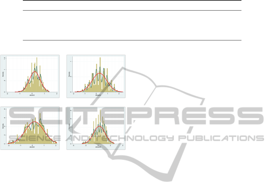
Table 4: Parameter estimates for the regression of fuzzy outputs on the means of the value labels.
Dependent β
0
SE(β
0
) t(b
0
= 0) β
1
SE(β
1
) t(b
1
= 1) R
2
Het
∗
SET CoM3 -1.54 0.004 -420.2 1.293 0.001 487.1 0.946 0
SET MoM3 -0.947 0.007 -134.6 1.205 0.001 177.7 0.806 0
SET CoM4 -3.622 0.006 -562.6 1.577 0.001 605.5 0.913 0
SET MoM4 -3.623 0.008 -473.1 1.637 0.001 506.7 0.866 0
∗ Breusch-Pagan / Cook-Weisberg test for heteroskedasticity, where H
0
is constant variance.
3-input mf / CoM 3-input mf / MoM
4-input mf / CoM 4-input mf / MoM
Figure 5: Distributions of differences between the fuzzy
outputs and the mean of the value labels (¯x
set;i
).
the consequent limitation of statistical data analysis of
ordinal, but also nominal variables. For example, the
use of the mean (sample average) becomes irrelevant
because the response of the FIS could be maintained
as ordinal. However, if a numerical output is desired,
as in the case-study presented here, then many prob-
lems still hold conceptually, but some of them are
operatively irrelevant as the vagueness weakens the
sharpness. In other words, by construction, the na-
ture of the fuzzy inputs mitigates the certainty that we
would normally have about the distances of the num-
bers on a given scale. Therefore, the issue concerning
the value attributed to a modality (e.g. 7 assigned to
“Yes rather than no” leading to questions like “Why 7
and not 7.5 or 6.5 or 8 or 6”) is less restrictive because
the fuzzification spreads the choice over the support,
even if all choices affect the output. In any case, the
FIS-based approach could represent a bridge between
qualitative and quantitative analysis for a consistent
treatment of concepts that are measured differently.
This potentiality would be useful in many fields of
application.
FIS, however, also presents difficulties at each
construction step. In the identification of the issue
(step i), the order in which the input variables are ag-
gregated in the system affects the output. Particularly,
input variables in the first nodes of the tree affect the
output less than those forming the subsequent nodes.
Moreover, the exponential explosion of the number
of rules limits the input of fuzzy modules to two or
three variables. The fuzzification of input (step ii) is
not a straightforward step and leaves a kind of inde-
terminacy. The construction of block rules (step iii)
is a subjective process open to criticism by all, as
there is no rule to make rules. In fact, the heuristic
fuzzy rules constitute a controversial issue. Certainly,
the flexibility derived from these rules allows for ad-
equately representing the actual phenomenon, but for
this same reason, the choices of the decision-maker
play a key role in the pattern of combinations involv-
ing the wording of the items. There are many meth-
ods and possibilities for the aggregation of block rules
(step iv), but they must be selected on the bases of the
knowledge of their functioning. Defuzzification (step
v) also offers a large variety of techniques that might
puzzle final users, although it can be seen as not being
a part of the core of a FIS or of the fuzzy set theory
(Van Leekwijck and Kerre, 1999).
Overall, the FIS generates reasonable and reliable
results, showing remarkable flexibility and more man-
ageability than the official evaluation systems, in spite
of discrepancies with respect to the means of the value
labels, which are the official results used by the per-
sons in charge of academic organization. However,
part of this manageability could originate from the
arbitrary choices required by the construction steps,
especially from the heuristic fuzzy rules (if – then
rules) and from the fuzzy inference method (selection
of aggregation’s operators for precondition and con-
clusion). Despite some unavoidable degree of arbi-
trariness in some modeling choices, the results were
satisfactory. The final outcomes resembled those of
the traditional procedure, but the values were slightly
higher than those of the official evaluations.
REFERENCES
Babbie, E. R. (2010). Introduction to social research. Cen-
gage learning, Wadsworth (Belmont, CA), 12th edi-
tion.
FuzzyInferenceSystemtoAnalyzeOrdinalVariables-TheCaseofEvaluatingTeachingActivity
35

Bernberg, R. E. (1952). Socio-psychological factors in in-
dustrial morale: I. the prediction of specific indicators.
The Journal of Social Psychology, 36(1):73–82.
Cantril, H. and Free, L. A. (1962). Hopes and fears for self
and country. American Behavioral Scientist, 6(2):4–
30.
CNVSU (2002). Proposta di un insieme minimo di do-
mande per la valutazione della didattica da parte degli
studenti frequentanti. Doc 09/02, Retrieved from
http://www.cnvsu.it:Accessed 28 July 2011.
Crespi, I. (1961). Use of a scaling technique in surveys. The
Journal of Marketing, 25(July):69–72.
Crespi, L. P. (1945a). Public opinion toward conscien-
tious objectors: Ii. measurement of national approval-
disapproval. The Journal of Psychology, 19(2):209–
250.
Crespi, L. P. (1945b). Public opinion toward conscien-
tious objectors: Iii. intensity of social rejection in
stereotype and attitude. The Journal of Psychology,
19(2):251–276.
Dubois, D. and Prade, H. E. (2000). Fundamentals of fuzzy
sets. Kluwer Academic Publishers, Boston, MA.
Grzegorzewski, P. (2008). Trapezoidal approximations of
fuzzy numbers preserving the expected interval – al-
gorithms and properties. Fuzzy Sets and Systems,
159(11):1354–1364.
Grzegorzewski, P. and Mr
´
owka, E. (2005). Trapezoidal ap-
proximations of fuzzy numbers. Fuzzy Sets and Sys-
tems, 153(1):115–135.
Grzegorzewski, P. and Mr
´
owka, E. (2007). Trapezoidal ap-
proximations of fuzzy numbers – revisited. Fuzzy Sets
and Systems, 158(7):757–768.
Juster, F. T. (1960). Prediction and consumer buying inten-
tions. The American Economic Review, 50(2):604–
617.
Juster, F. T. (1966). Consumer buying intentions and
purchase probability: An experiment in survey de-
sign. Journal of the American Statistical Association,
61(315):658–696.
Kilpatrick, F. P. and Cantril, H. (1960). Self-anchoring scal-
ing: A measure of individuals’ unique reality worlds.
Journal of Individual Psychology, 16(2 Nov):158–
173.
Lalla, M. and Facchinetti, G. (2004). Measurement and
fuzzy scales. Atti della XLII Riunione Scientifica,
pages 351–362.
Lalla, M., Facchinetti, G., and Mastroleo, G. (2004). Or-
dinal scales and fuzzy set systems to measure agree-
ment: An application to the evaluation of teaching ac-
tivity. Quality and Quantity, 38(5):577–601.
Lalla, M. and Ferrari, D. (2011). Web-based versus paper-
based data collection for the evaluation of teaching ac-
tivity: empirical evidence from a case study. Assess-
ment & Evaluation in Higher Education, 36(3):347–
365.
Likert, R. (1932). A technique for the measurement of atti-
tudes. Archives of psychology, monograph no. 140:1–
55.
Marsh, H. W. (1987). Students’ evaluations of university
teaching: Research findings, methodological issues,
and directions for future research. International jour-
nal of educational research, 11(3):253–388.
N.N. (2007). fuzzyTECH 5.7 Users Manual. INFORM
GmbH, Aachen, D.
Osgood, C. E. (1952). The nature and measurement of
meaning. Psychological bulletin, 49(3):197–237.
Osgood, C. E., Suci, G. J., and Tannenbaum, P. H. (1957).
The measurement of meaning. University if Illinois
Press, Urbana, IL.
Schuman, H. and Presser, S. (1996). Questions and an-
swers in attitude surveys: Experiments on question
form, wording, and context. Sage Publications, Thou-
sand Oaks, CA.
Smithson, M. (1988). Fuzzy set theory and the social sci-
ences: the scope for applications. Fuzzy Sets and Sys-
tems, 26(1):1–21.
Stevens, S. S. (1946). On the theory of scales of measure-
ment. Science, 103:677–680.
Thurstone, L. L. (1927). A law of comparative judgment.
Psychological review, 34(4):273–286.
Thurstone, L. L. (1928). Attitudes can be measured. Amer-
ican journal of Sociology, 33(4):529–554.
Van Leekwijck, W. and Kerre, E. E. (1999). Defuzzifica-
tion: criteria and classification. Fuzzy sets and sys-
tems, 108(2):159–178.
Von Altrock, C. (1997). Fuzzy logic and neuroFuzzy appli-
cations in business and finance. Prentice Hall PTR,
Upper Saddle River, NJ.
Weisberg, H. F. and Rusk, J. G. (1970). Dimensions of can-
didate evaluation. The American Political Science Re-
view, 64(4):1167–1185.
White, M. (1926). Psychological technique and social
problems. Southwestern Political and Social Science
Quarterly, 7:58–73.
Yeh, C.-T. (2009). Weighted trapezoidal and triangular ap-
proximations of fuzzy numbers. Fuzzy Sets and Sys-
tems, 160(21):3059–3079.
Yu, J. H., Albaum, G., and Swenson, M. (2003). Is a central
tendency error inherent in the use of semantic differ-
ential scales in different cultures? International Jour-
nal of Market Research, 45(2):213–228.
FCTA2014-InternationalConferenceonFuzzyComputationTheoryandApplications
36
