Adaptive Output Feedback Controller with Operating Constraints

for Solid Oxide Fuel Cells

Lei Pan

, Chengyu Cao

and Jiong Shen

School of Energy and Environment, Southeast University, 2 Si Pai Lou Road, Nanjing, China

Department of Mechanical Engineering, University of Connecticut, Storrs, U.S.A.

Keywords: L

Adaptive Controller, Solid Oxide Fuel Cell, Constraints, Disturbance Model Predictive Controller.

Abstract: Control on solid oxide fuel cells (SOFC) is challenging due to its nonlinearity, time-varying uncertainties,

tight operating constraints and modeling difficulties. The L

adaptive output feedback controller for systems

of unknown relative degree is introduced for the SOFC output voltage control in this paper. It allows for fast

and robust adaptation, and provides improved transient performance. Its advantages of not enforcing a

strictly positive real condition along with the low-pass filtered control signal bring it the potential to be

applied in wide industrial processes. In the study of the SOFC control, a dynamic SOFC model is first built;

then a L

adaptive output feedback controller is designed only using the nominal working conditions of the

SOFC model. Through setting the operating constraints at proper locations, the closed-loop stability is

maintained in the presence of hard constraints by the symmetric structure of the L

adaptive control loop. A

simulation comparison is made in the SOFC constant voltage control process between the L

adaptive

controller and a linear disturbance model predictive controller (DMPC) for their almost equal complexity in

designs. The result shows the advantage of the L

adaptive controller in disturbance rejections for its faster

transient response.

1 INTRODUCTION

Solid oxide fuel cell (SOFC) is a kind of high

efficiency, environment friendly power generation

assembly, which converts the chemical energy in

fuel and oxidant directly to electricity. Because of

the shortage of resources and increasing

environment pollutions, governments and

technicians all over the world pay more attentions on

the research and development of SOFC today. SOFC

in the application of massive distributed power

sources has been considered to be a potential

candidate to replace the traditional thermal cycle

power generation. The SOFC system has severe

output nonlinearity and tight operating constrains. It

also has time-varying uncertainties and is hard to

model. These features bring the major challenges on

the control methods of SOFC systems. Because

effective control on SOFC system can improve

operation efficiency, extend the stack lifespan, and

improve the quality of power, more and more

research has been taken on designing high-

performance controllers working with nonlinear and

uncertain dynamic characteristics of SOFC plants in

recent years.

Most of the research work is based on model

predictive control (MPC) methods (Pukrushpan et

al., 2002; Vahidi et al., 2004; Aguiar et al., 2005;

Stiller et al., 2006). The conventional MPC is a

receding-horizon linear quadratic control law, but it

can be extended for nonlinear control by

incorporating nonlinear prediction models. Fuzzy

prediction models and data-driven prediction models

are mainly used in nonlinear SOFC predictive

controls. A fuzzy Hammerstein model is used as the

predictive control model to achieve online control of

an SOFC system (Huo et al., 2008). In order to

control the stack temperature of a SOFC within a

safe range, an online nonlinear MPC scheme based

on an improved T-S fuzzy model is proposed (Yang

et al., 2009). Its control sequence could be obtained

by the branch-and-bound method. The nonlinear

predictive controller based on an improved radial

basis function neural network is applied (Wu et al.,

2008). It controls the voltage and guarantees fuel

utilization within a safe range and uses the genetic

algorithm for parameter optimizations. In order to

reduce the heavy computing load in nonlinear MPC

499

Pan L., Cao C. and Shen J..

L1 Adaptive Output Feedback Controller with Operating Constraints for Solid Oxide Fuel Cells.

DOI: 10.5220/0005043604990507

In Proceedings of the 11th International Conference on Informatics in Control, Automation and Robotics (ICINCO-2014), pages 499-507

ISBN: 978-989-758-039-0

 2014 SCITEPRESS (Science and Technology Publications, Lda.)

control, which is mainly caused by the nonlinear

optimization and on-line model identifications, the

disturbance model predictive control (Muske and

Badgwell, 2002) is introduced for SOFC (Pan and

Shen, 2012). It has less computing load and can deal

with some nonlinearity and uncertainty

characteristics. But it is non-adaptive and cannot

guarantee the closed-loop stability while achieving a

fast disturbance-rejection.

In this paper, we try to introduce another

advanced control approach, L

adaptive control, for

designing the SOFC control system. L

adaptive

control offers its own set of attractive features,

including fast and robust adaptation. In addition to

the conventional asymptotic performance

characterization, L

adaptive control permits

transient analysis for both control signal and system

response. Furthermore, this methodology has been

extended to systems with unknown time-varying

parameters (Cao and Hovakimyan, 2007), to systems

with nonlinear uncertainties (Cao and Hovakimyan,

2008), to systems with un-modeled internal and

actuator dynamics (Cao and Hovakimyan, 2008), to

systems in the presence of non-zero trajectory

initialization error (Cao and Hovakimyan, 2008),

and to a certain output feedback framework (Cao

and Hovakimyan, 2009). L

adaptive control has

been very successfully applied in unmanned flight

controls which have nonlinearities, time-varying

disturbances, unknown parameters and un-modeled

dynamics.

An extension approach of the L

adaptive output

feedback control (Cao and Hovakimyan, 2009) to

systems of unknown relative degree may deal well

with the control problems of SOFC, e.g., time-

varying uncertainties with unknown rate of

variations caused by load disturbances. Compared to

other L

adaptive control methods, this approach

adopts a new piece-wise continuous adaptive law

along with the low-pass filtered control signal. It

allows for achieving arbitrarily close tracking of the

reference signals, and the transfer function of its

reference system is not required to be strictly

positive real (SPR). Stability of this system is

guaranteed by its design via small-gain type

argument. These features show that this L

adaptive

control approach may have great potential to be

applied in wide industrial processes.

In this paper, we reproduce a SOFC simulation

model as the plant; then take advantage of its

nominal working conditions to design a L

adaptive

output feedback controller. Through the analysis on

the controller framework, the operating constraints

are set to the proper position in the loop. It holds the

closed-loop stability in the presence of the hard

constraints. Simulations comparing to a linear

disturbance model predictive controller (DMPC) on

the SOFC model show that L

adaptive control has

better disturbance-rejection performance and much

faster temporary regulating-process on the SOFC

constant voltage.

The paper is organized as follows. Section 2

describes the dynamic SOFC model. In Section 3, L

adaptive output feedback controller with operating

constraints is designed. For making an evaluation on

the new controller, a linear DMPC controller is

designed in Section 4. The simulation results along

with some discussions on these two SOFC control

methods are presented in Section 5. Section 6

concludes the paper.

2 DYNAMIC MODEL OF SOFC

Many nonlinear dynamic models of SOFC with

detailed descriptions on cell internal processes are

too complicated to support a controller designing

process. The model reported in the paper (Padullés

and Ault, 2000) describes the key characteristics of

the SOFC dynamic process in the Laplace transform

domain. It shows challenging control problems

owing to SOFC’s nonlinear dynamics, tight

operating constraints and unexpected disturbances. It

has been taken as a benchmark commonly studied in

the SOFC control literature (Huo et al., 2008; Wu et

al., 2008; Yang et al., 2009). Therefore, this model

will be adopted as the SOFC plant for the L

adaptive

controller design. Some preconditions (Padullés and

Ault, 2000) are stated in the following: The gases

are ideal; The stack is fed with hydrogen and air;

The flow ratio of hydrogen to oxygen is kept at

1.145; Lump gas pressures are considered in the

channels along the electrodes; The temperature is

stable; The exhaust of each channel is via a single

orifice, and the ratio of pressures between the

interior and exterior of the channel is large enough

to consider that the orifice is choked; The Nernst

equation can be applied. This dynamic SOFC model

consists of the fuel processor and the fuel cell stack,

as shown in Fig. 1, where E denotes the stack output

voltage (V), q

the natural gas flow rate (mol/ s), and

I the external current load (A); p

, p

, and p

H2O

denote the partial pressures (Pa) of hydrogen,

oxygen, and water, respectively; q

H2,in

and q

O2,in

are

the input flow rates of hydrogen and oxygen (mol/s),

respectively. The model is described in the

following and all the parameters are annotated in

Table 1.

ICINCO2014-11thInternationalConferenceonInformaticsinControl,AutomationandRobotics

500

2.1 The Fuel Processor

The fuel processor converts fuels such as natural gas

to hydrogen and byproduct gases. From the

viewpoint of control analysis, a first-order transfer

function with time constant



can well describe the

dynamic reform process from the natural gas input

to the hydrogen-rich fuel q

,in

. The fuel processor

can be simply represented by

H2,in







(1)

Hydrogen reacts with oxygen in SOFC and

generates water. The flow ratio between hydrogen

and oxygen is represented by

Oin







(2)

For having a complete reaction by the excessive

oxygen, take the ratio



H-O

as 1.145 (Padullés and

Ault, 2000).

2.2 The Fuel Cell Stack

Applying Nernst’s equation and taking into account

ohmic, concentration, and activation losses (i.e.,



and



), the stack output voltage is given by

( /101325)

oca

ENE







 





(3)

Where

(2)

HHr

qKI









(4)

()

OOr

qKI









(5)

HO r

pKI









(6)

log







(7)

ln 1

RT I





 





(8)





(9)

Equation (4)-(6) represent the dynamic

characteristics of the partial gas pressure of

hydrogen, oxygen and water inside the anode

channel associated with their molar flows through

the anode valve respectively. Take hydrogen as an

example to derive it. Consider the molar flow of

Hydrogen is proportional to its partial pressure

inside the channel and have



(10)

Take time derivative on the perfect gas equation of

hydrogen and obtain

2, 2, 2,

()

in H o H r

qqq

dt V



(11)

Where q

H2,in

is the input hydrogen flow, q

H2,o

is the

output hydrogen flow, and q

H2,r

is the hydrogen flow

that reacts. According to the basic electrochemical

relationships, q

H2,r

can be calculated by

Hr r

qKI



(12)

Apply (10) and (12) in (11) and then take the

Laplace transform, obtaining (4) and the equation

/( )

VKRT





The transfer functions of oxygen and steam are

derived as well.

The fuel utilization which is one important

operating variable and may affect the performance

of SOFC is defined as

2, 2, 2,

Hin HO Hr

in H in H in

qq q

qqFq





(13)

The desired range of fuel utilization is from 0.7 to

0.9. The overused (u

> 0.9) and underused (u

< 0.7)

fuel conditions should be prevented. An overused

condition could lead to permanent damage to the

cells due to fuel starvation and an underused-fuel

situation results in unexpectedly high cell voltages

(Vahidi et al., 2004).











2,Hin

2,Ho



















( /101325)











2HO

Figure 1: Dynamic model of SOFC.

Table 1: Parameters of the SOFC.

Para-

meter

Value Representation

T 1273 K Absolute temperature

F 96,485 C /mol Faraday’s constant

8.314

J/(mol·K)

Universal gas constant

1.18 V Ideal standard potential

384

Number of cells in

series in the stack

0.996×10

−3

mol/(s·A)

Constant, Kr =N

/4F

L1AdaptiveOutputFeedbackControllerwithOperatingConstraintsforSolidOxideFuelCells

501

Table 1: Parameters of the SOFC. (Cont.)

Para-

meter

Value Representation

8.32 × 10

−6

mol/(s·Pa)

Valve molar constant

for hydrogen

H2O

2.77 × 10

−6

mol/(s·Pa)

Valve molar constant

for water

2.49 × 10

−5

mol/(s·Pa)

Valve molar constant

for oxygen



26.1 s

Response time of

hydrogen flow



H2O

78.3 s

Response time of water

flow



2.91 s

Response time of

oxygen flow



H−O

1.145

Ratio of hydrogen to

oxygen

r 0.126 Ω Ohmic loss



5 s

Time constant of the

fuel processor

∂ 0.05 Tafel constant



0.11 Tafel slope

800 A

Limiting current

density

3 L

ADAPTIVE CONTROLLER

WITH INPUT CONSTRAINTS

ON SOFC

Several aspects should be considered in the design

of a controller for the SOFC system.

First, we know from the modeling work in

Section 2 that the nonlinear SOFC model composed

of (1) to (13) has the Wiener-type output

nonlinearity. Suppose the operating temperature and

pressure of the SOFC is kept constant, then the stack

terminal voltage E is mainly influenced by the inlet

hydrogen flow q

H2,in

and the current I. The operating

stack voltage usually shows significant changes at

low and high current loads, even shows a rapid

deterioration caused by overloaded current. Thus the

stack current is often taken as the main disturbance

variable to the process.

Second, the feasible operation area of SOFC

shows that it is impossible for SOFC to maintain a

simultaneous constant fuel utilization u

and constant

output voltage E operating regime for a range of

current I. The constant voltage control is much safer

than the constant fuel utilization control for the fuel

utilization performs (Wu et al., 2008).

In order to achieve a constant stack voltage

control under drastic current load disturbances, a L

adaptive output feedback controller is designed for

keeping both the SOFC output voltage at set point

and the fuel utilization within the safe range. Fig.2

shows the structure of the L

adaptive output

feedback control loop for a SOFC process.

()yt

()t



Figure 2: L

Adaptive output feedback control system for

SOFC.

3.1 Problem Formulation

Describe the controlled SOFC voltage dynamics as

the following single-input single-output system:

() ()(() ())ys As us ds





(14)

where yR is the SOFC terminal voltage, uR is the

hydrogen flow rate, A(s) is a strictly proper

unknown transfer function of unknown relative

degree nr, for which only a known lower bound 1<

dr <nr is available, d(s) is the Laplace transform of

the time-varying uncertainties and disturbance d(t) =

f(t, y(t)), where f is an unknown map, subject to the

following assumption:

Assumption 1 There exist constants L>0 and

>0 such that for all t≥0:

1212

(, ) (, )

ty fty Ly y

(15)

(, )

ty Ly L





(16)

Assumption 2 There exist constants L

>0, L

and L

>0 such that for all t≥0:

123

() ()dLyt Lyt L







(17)

where the numbers L, L

, L

can be

arbitrarily large.

Assumption 3 The DC gain of the nominal

working point of SOFC is known.

Let r(t) be a given bounded continuous reference

input signal. The control objective is to design an

adaptive output feedback controller u(t) such that the

system output y(t) tracks the reference input r(t)

following a desired reference model

() ()()ys Msrs



(18)

where M(s) is a minimum-phase stable transfer

function of relative degree dr > 1. Thus we can

rewrite the system in (14) as:

ICINCO2014-11thInternationalConferenceonInformaticsinControl,AutomationandRobotics

502

() ()(() ())ys Ms us s



 (19)

() (( () ())() () ())/ ()

As Ms us Asds Ms



  (20)

Let (A

 R

NN

, b

 R

, c

 R

) be the minimal

realization of M(s). Thus the system in (19) can be

rewritten as:

() () ( () ())

() (), (0)

tAxtbut t

yt c xt x x



 





(21)

3.2 L

Adaptive Output Feedback

Controller

Adaptive controller consists of the state predictor,

the adaptation law and the control law.

The state predictor is given by:

ˆˆ ˆ

() () () ()

ˆˆ

() (), (0)

tAxtbut t

yt c xt x x









(22)

Where

()

t  R

and

()yt

 R are the state and

output of the predictor respectively;

()t



 R

compensates the system disturbances and model

mismatch. It is on-line estimated by the following

adaptation law:

ˆˆ

() ( ) [ ,( 1) ],

() ()(), 0,1,2, ,

tiTtiTiT

iT T iT i









  

(23)

Where T>0 is the sampling time of the adaptation

law; and

()

( ) 1 ( ), 0,1, 2, .

Te d

iT e y iT i







 















(24)

Where 1

 R

be the basis vector with first element

1 and all other elements zero;

() () (); ,

yt yt yt R





 









where P=P

>0 satisfies the algebraic Lyapunov

equation A

P + PA

= -Q, Q>0; and let D  R

(N-

1)N

satisfies

(( )) 0

Dc P





The control law is defined via the output of the

low-pass filter C(s):

()

() ()() ( ) ()

()

us Csrs c SI A s





 

(25)

The selection of C(s) and M(s) must ensure that

() () ()/( () () (1 ()) ())H s AsM s Cs As Cs M s

(26)

is stable and that the L

-gain of the system is

bounded as follows:

()(1 ()) 1

Hs Cs L





(27)

(Cao and Hovakimyan, 2009).

The above piece-wise continuous adaptive law

with the low-pass filtered control signal allows for

achieving arbitrarily close tracking of the input and

the output signals of the reference system. The

performance bounds between the closed-loop

reference system and the closed-loop L

adaptive

system can be rendered arbitrarily small by reducing

the step size of integration. It can be represented by

the following equations.

lim ( ) ( ), lim ( ) ( )

ref ref

yt y t ut u t





where T is the integration step of the L

adaptive

controller.

3.3 Operating Constraints for SOFC

Besides the design above, we need to put the input

constraints in the L

adaptive controller for the

SOFC voltage control, i.e., letting

min max

()uutu

hold for all t≥0, where u

min

=0, u

max

=1.7023mol/s

given in the paper (Padullés and Ault, 2000).

Considering the subtle symmetric structure of L

adaptive control, we cannot constrain u(t) directly.

()t



is sent into both the plant and the state

predictor for cancellation. Its constraints can

influence the value of u(t) but cannot change the

stability of the closed loop. Thus, we have

min max

min min

max min

ˆˆ ˆ

(), ()

ˆˆ ˆ

() , ( )

ˆˆ

,()

[,( 1)], 0,1,2,.

iT if iT

tifiT

if iT

tiTi T i



 

















 

(28)

Another point is the possible different DC gains

between the plant and the state estimator. Because

the nominal parameters of SOFC are available, we

have Assumption 3. Dividing the output voltage

reference by the nominal DC gains of the SOFC

system, we get r(t) in control law (25).

4 DMPC CONTROLLER DESIGN

FOR A COMPARISON

In order to evaluate the performance of the L

Adaptive controller for SOFC, we try to introduce

L1AdaptiveOutputFeedbackControllerwithOperatingConstraintsforSolidOxideFuelCells

503

the linear disturbance model predictive controller

(Muske and Badgwell, 2002; Pannocchia and

Rawlings, 2003) to be an evaluating reference. It is a

kind of target-adaptive offset-free MPC with the

advantages in disturbance rejection and offset-free

tracking. The DMPC has been successfully applied

in CSTR (Pannocchia and Rawlings, 2003) and

become a fundamental approach where a variety of

MPC approaches have derived. The L

Adaptive

controller and the DMPC controller have almost

equal complexity in designs and computation load

online, therefore we will compare their performance

in the simulations. For clarity, a brief design of the

DMPC controller for SOFC is presented. First, the

augmented disturbance prediction model of SOFC is

built in term of the conditions for detectability, and

then the problem of estimating the augmented

disturbance states is solved. As a result, an

augmented observer is used to estimate the system

states and the lumped mismatch. Last, the

augmented disturbance model is adopted in the

predictive control algorithm to realize the control of

SOFC.

4.1 Disturbance Model and Estimator

We need to describe the SOFC plant approximately

by a linear model with augmented disturbance states

before the design of the DMPC controller. The

following linearized discrete state-space model

describes the controlled voltage system

1kkk

Gx Hu

yCx







(29)

where y R is the SOFC terminal voltage, u R is

the hydrogen flow rate, x  R

is the process state

and its rank represents the inertial of the process,

G R

22

, H R

21

, C R

12

, (G, H) is stabilizable

and (C,G) is detectable in the SOFC model. There

must be some model-plant mismatch in using the

linear model of Eq.29. We lump the mismatch along

with load disturbances into an augmented state to

make a disturbance model of SOFC



01 0

GG H

yCC



 





 





 









(30)

where d R, G

 R

21

, C

 R

11

. Because the

lumped disturbance is unmeasured, an estimator is

needed for state-observing

1| | 1

|1 |1

ˆˆ

01 0

()

kk kk

kkk dkk

GG H

yCx Cd





 



 

 

 

 









(31)

where L

 R

21

, L

 R

11

are the predictor gain

matrices for the state and the disturbance. Since the

additional modes introduced by the disturbance are

unstable, detectability of the augmented system is a

necessary and sufficient condition for a stable

estimator to exist.

4.2 Detectability of the Augmented

State Space

The condition which ensures the observability of the

augmented disturbance system is given in the

following Lemma (Muske and Badgwell, 2002).

Lemma The augmented system presented in Eq.

30 is detectable if and only if (C,G) is detectable and

()

IG G

rank n n











(32)

Where n is the number of the nonaugmented states,

is the number of the disturbances. In the SOFC

system, n is 2 and n

is 1. This Lemma implies that

the maximum dimension of the disturbance d in

Eq.30 such that the augmented system is detectable

is equal to the number of measurements y. That

gives us the guideline to design the augmented

system. Because (C, G) is detectable, the disturbance

model is defined by choosing the matrices G

and C

to hold Eq.32.

4.3 Target-adaptive MPC Algorithm

The goal of tracking the steady-state target is to

remove the effects of the estimated constant

disturbance states in the MPC control. It is a kind of

target-adaptive control. Given the current estimate of

the disturbance

d , the state and input target are

computed by solving the following quadratic

program

min max

min | max

min( ) ( )

ts ts

dkk

dkk s

tdkk

uu Ruu

IG H

Cd y

uuu

yCxCdy



































 

(33)

ICINCO2014-11thInternationalConferenceonInformaticsinControl,AutomationandRobotics

504

where x

 R

, u

 R, R

’

 R and R

’

>0, y

 R

and

 R are the setpoints of the controlled and

manipulated variables respectively.

By tracking the steady-state target of the

manipulated variable, the MPC controller solves the

following optimization problem to obtain the input

sequence

, ,...

min max

min ( ) ( )

()()

.. .30

ks ks

kt kt

yyQyy

uuRuu

st Eq

uuu

yyy





 

 





(34)

where Q  R

and R  R

With an augmented disturbance prediction model

of SOFC and an online target-optimization

algorithm, the DMPC controller can deal with the

plant-model mismatch, unmodeled plant

disturbances and achieve the zero offset output

tracking. The design complexities of DMPC and L

adaptive controller are at the same level.

5 SIMULATIONS

AND DISCUSSION

Design the L

adaptive output feedback controller

based on (22)-(25) for the SOFC model shown in

Fig.1. The design information is shown as follows.

The reference model

()

1.4 1





; the filter

()

25 9





; the sampling interval T=0.01s; the

offset range

min



= -0.4,

max



=0.4; the variables at

the nominal working point, I=300A, q

=0.746mol/s,

E=341.7V.Only the nominal DC gain of the SOFC

process is used for designing the L

adaptive

controller. Modeling is not needed for this control

algorithm.

Because of its successful and wide applications,

the model predictive control approach can act as a

reference to evaluate the L

adaptive output feedback

controller. Considering there are many kinds of

MPC approaches, we choose two ways to make

these comparisons.

First, the linear offset-free disturbance model

predictive controller (DMPC) presented in Section 4

is adopted for the comparison with the L

adaptive

output feedback controller. We apply L

adaptive

controller and DMPC controller respectively on the

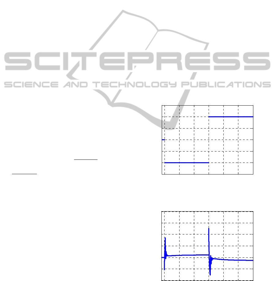
SOFC model. We put two step disturbances into the

simulation experiments. Assuming at t = 400 s, a

load disturbance causes the stack current to have a

step change (from 300 to 280 A), and at t = 700 s, a

load disturbance causes the stack current to have

another step change (from 280 to 320 A). The step

disturbances on the stack current are shown in Fig.

3(a). Fig. 3(b) shows the fuel utilization by L

adaptive control. It is kept within the safe range. Fig.

3(c) and Fig. 3(d) compare the curves of the constant

voltage by L

and DMPC control. It shows that the

adaptive control has a shorter temporary

regulating-process in the constant voltage control.

For improving the robustness, the regulating of

DMPC is much slower than that of L

adaptive

control, which can be seen from the control signal

shown in Fig.3(e) and Fig.3(f). If we quicken the

DMPC regulating, the DMPC control system may

not be stable. Thus, L

adaptive control has obvious

advantages over DMPC control in the fast tracking

and disturbance rejection in this case. Something to

note, we cannot say the control performance of

DMPC shown in Fig.3 is its best one, but it is its

best in all our simulations.

400 500 600 700 800 900 1000

270

280

290

300

310

320

330

time (s)

Current

I(A)

(a) Disturbance of stack current.

400 500 600 700 800 900 1000

0.7

0.75

0.8

0.85

0.9

0.95

time (s)

Fuel Utilization

(b) From L

adaptive control.

L1AdaptiveOutputFeedbackControllerwithOperatingConstraintsforSolidOxideFuelCells

505

400 500 600 700 800 900 1000

330

335

340

345

350

Output Voltage

time (s)

E(V)

adaptive control.

400 500 600 700 800 900 1000

330

332

334

336

338

340

342

344

346

348

350

Output Voltage

time (s)

E(V)

(d) From DMPC control.

400 500 600 700 800 900 1000

0.5

0.6

0.7

0.8

0.9

time (s)

Input Hydrogen flow

mol/s

(e) From L

adaptive control.

400 500 600 700 800 900 1000

0.5

0.55

0.6

0.65

0.7

0.75

0.8

0.85

0.9

0.95

Input Hydrogen flow

time (s)

mol/s

(f) From DMPC control.

Figure 3: The simulation results of the

adaptive control

and DMPC control on SOFC process.

Second, some comparisons are made with other

published results of a nonlinear MPC (Li et al.,

2011), we find that the L

adaptive controller has a

better rapidness under the guaranteed stability in the

nonlinear SOFC process control and has much less

online computation load.

6 CONCLUSIONS

This paper illustrates the fast-adaptation L

adaptive

controller design for the nonlinear SOFC process

control. An output feedback controller is designed

for SOFC system with unknown dynamics. Unlike

model-based control, it only needs a few system

parameters to design. The simulation results show

that it has good capability of disturbance rejection

and fast reference-tracking.

ACKNOWLEDGEMENT

The authors are grateful to the support of the

National Natural Science Foundation of China under

Grants 51106024 and 51036002. The authors would

like to express their appreciations to all the

reviewers for their invaluable comments.

REFERENCES

Aguiar, P., Adjiman, C., Brandon, N., 2005. Anode-

supported intermediate temperature direct internal

reforming solid oxide fuel cell: II. Model-based

dynamic performance and control. J. Power Sources,

147(1-2), 136-147.

ICINCO2014-11thInternationalConferenceonInformaticsinControl,AutomationandRobotics

506

Cao, C., Hovakimyan, N., 2007. Guaranteed transient

performance with L

adaptive controller for systems

with unknown time-varying parameters: part I.

Proceedings of American Control Conference, New

York.

Cao, C., Hovakimyan, N., 2008. L

adaptive controller for

a class of systems with unknown nonlinearities: part I.

American Control Conference, Seattle, WA.

Cao, C., Hovakimyan, N., 2008. L

adaptive controller for

nonlinear systems in the presence of unmodelled

dynamics: Part II. American Control Conference,

Seattle, WA.

Cao, C., Hovakimyan, N., 2008. L

adaptive controller for

systems with unknown time-varying parameters and

disturbances in the presence of non-zero trajectory

initialization error. International Journal of Control,

81(7), 1147–1161.

Cao, C., Hovakimyan, N., 2009. L

adaptive output

feedback controllers for non-strictly positive real

reference systems: missile longitudinal autopilot

design. Journal of Guidance, Control, and Dynamics,

32(3), 717-726.

Huo, H. B., Zhu X.J., Hu, W. Q., Tu, H. Y., Li, J., Yang,

J., 2008. Nonlinear model predictive control of SOFC

based on a Hammerstein model. J. Power Sources,

185(1), 338-344.

Li Y. G., Shen J., Lu J. H., 2011. Constrained model

predictive control of a solid oxide fuel cell based on

genetic optimization. J. Power Sources, 196, 5873-

5880.

Muske, K. R., Badgwell, T. A., 2002. Disturbance

modeling for offset-free linear model predictive

control. J. process control, 12(5), 617-632.

Padullés, G. W., Ault, J. R., 2000. An integrated SOFC

plant dynamic model for power systems simulation. J.

Power Sources, 86(1-2), 495-500.

Pan, L., Shen, J., 2012. Disturbance modeling and offset-

free predictive control for solid oxide fuel cell. 55th

ISA POWID Symposium, 492, 293-307.

Pannocchia, G., Rawlings, J. B., 2003. Disturbance

models for offset-Free model-predictive control.

AIChE Journal, 49(2),426-437.

Pukrushpan, J., A. Stefanopoulou, Peng, H., 2002.

Modeling and control for pem fuel cell stack system.

In Proc. of the 2002 American Control Conf.,

Anchorage, AK, pp. 3117-3122.

Stiller, C., Thorud, B., Bolland, O., Kandepu, R., Imsland,

L., 2006. Control strategy for a solid oxide fuel cell

and gas turbine hybrid system. J. Power Sources,

158(1), 303-315.

Vahidi, A., Stefanopoulou, A., Peng, H., 2004. Model

predictive control for starvation prevention of a hybrid

fuel cell system. In Proc. of the 2004 American

Control Conf., Boston, MA, 834-839.

Wu, X. J., Zhu, X.J., Cao, G.Y, Tu, H.Y., 2008. Predictive

control of SOFC based on a GA-RBF neural network

model. J. Power Sources, 179(1) , 232-239.

Yang, J., Mou, H. G., Li, J., 2009. Predictive control of

solid oxide fuel cell based on an improved Takagi-

Sugeno fuzzy model. J. Power Sources. 193(2), 699-705.

L1AdaptiveOutputFeedbackControllerwithOperatingConstraintsforSolidOxideFuelCells

507