A Real-time Motion Data Reduction and Restoration Compatible with

Robot’s Physical Limits

Doik Kim, Jung-Min Park and Seokmin Hong

Interaction and Robotics Research Center, KIST,

Hwarangno 14-gil 5, Seongbuk-gu, Seoul, 136-791, Republic of Korea

Keywords:

Data Reduction, Restoration, Hardware Limit, Convolution Interpolation.

Abstract:

In order to control a robot, motion data obtained from various interface devices such as haptic and tele-

operating interfaces, and a motion capture system, or from predeﬁned parametric equations are needed. It is

hard to store and transmit the data because of their high control frequency and synchronization problem. In

addition, usually, all these data are only for one target robot system, i.e., it is hard to use them to other robot

system with different hardware limits. In order to solve the problems, the reduction of the original data is

conducted with two stage magnitude quantization and the restoration without violating the hardware limits,

such as maximum velocity, acceleration, etc., is conducted with the convolution interpolation, in this paper.

The proposed method can be used in on-line data transmission and for off-line data storage.

1 INTRODUCTION

A robot is controlled by motion data obtained from

various interface devices of tele-operation, haptics,

and motion capture system as well as parametric

equations for trajectory generation. If motion data are

to be stored for replaying later or to be transmitted to

remote devices in real-time, several problems need to

be considered. Especially the realtimeness, and target

system’s physical limits are essential to be considered

for stable and safe control.

Data size for controlling a robot is different

from robot to robot, according to its control Hz,

DOF(Degree of Freedom), control variables, etc. Ab-

solute size of motion data is less than other types of

data such as audio and video, but it must be guar-

anteed a real-time synchronization from sensors to

actuators through networks within its control sam-

pling time. This hard real-time condition makes

load of the network comparable to audio and video

data(Hinterseer et al., 2008).

In addition, the transmitted signal should not vi-

olate physical hardware limits such as velocity, ac-

celeration, jerk, etc. In many cases, the transmit-

ted data will be used for the same robot hardware

system, but if motion data are stored as reference

data, they can be applied to other robot hardware

systems as far as they are compatible to the original

robot. Compatibility can be qualiﬁed by consider-

ing workspace, DOF, structural similarity, and actu-

ation hardware limits, etc. For example, if two robots

have similar workspace and motion data for control

are composed of the position and orientation of the

end-effector, there is high possibility that the motion

data are compatible between two robots regardless of

their structures and DOF from the theoretical view-

point. However, in order to share the motion data

between real robot systems, the restored data should

not violate physical hardware limits of a target robot;

otherwise they make the robot unstable. Thus, non-

violation of physical hardware limits is a fundamental

condition for safe and stable control.

In order to solve the realtimeness, data reduc-

tion/restoration methods have been studied. Most re-

search is focused on the haptic data reduction and

transmission. DPCM(differential pulse code modu-

lation) related methods are used to reduce haptic mo-

tion data by (Shahabi et al., 2002; Kron et al., 2004).

Hirche, et al., proposed a psychophysically motivated

compression method with the deadband concept to re-

duce the haptic data(Hirche et al., 2007; Hirche and

Buss, 2007). If the difference between the current

data and the most recently transmitted data exceeds

a predeﬁned perception threshold (the deadband), the

current data are transmitted, and otherwise the haptic

data are abandoned. It is extended to 3 DOF haptic de-

vices in (Hinterseer et al., 2008), and 6-DOF in (Sakr

et al., 2010; Sakr et al., 2011) A haptic data reduction

360

Kim D., Park J. and Hong S..

A Real-time Motion Data Reduction and Restoration Compatible with Robot’s Physical Limits.

DOI: 10.5220/0005041303600367

In Proceedings of the 11th International Conference on Informatics in Control, Automation and Robotics (ICINCO-2014), pages 360-367

ISBN: 978-989-758-040-6

 2014 SCITEPRESS (Science and Technology Publications, Lda.)

based on human perception is summarized in (Stein-

bach et al., 2011). All these are concerned on the real-

timeness by reducing motion data, especially in tele-

presence and tele-action system, and thus human per-

ception is an important aspect in reducing data. How-

ever, from the viewpoint of control, human percep-

tion is a sub-condition of motion data reduction, i.e.,

motion data can be reduced more beyond the human

perception to control a robot, and it has not been con-

sidered deeply.

In the case of restoration, physical hardware lim-

its are not considered importantly, because the data

is used for the same hardware. However, if a set of

motion data is transmitted to or stored for later us-

age of several different robots, physical hardware lim-

its must be considered for safe and stable operation.

This discordance between source motion data and tar-

get robots cannot be solved in all cases, but in many

cases, it can be relaxed and increase the compatibility

in restoration stage by considering hardware limits.

To solve these realtimeness and hardware com-

patibility problems, two-stage data reduction and

convolution-based data restoration are proposed as

follows: section 2 and 3 describe the reduction and

restoration method, respectively. Section 4 shows ex-

perimental results, and section 5 concludes this paper.

2 DATA REDUCTION WITH

MINIMAL SHAPE

INFORMATION

Motion data are considered as set of signals having

similar properties such as noise level, sampling time,

etc. Speciﬁcally, motion data such as position, orien-

tation, joint angles, which are mostly used for control-

ling a robot and feeding the status back to a user, are

considered in the paper and other kinds of data can

also be considered similarly without any problem.

Original Data

Stage 1

Anchor Point

g=1

Stage 2

Deadband

Reduced data

Change

Reduction level

0 <= g < 1

Yes

Ignore

Figure 1: Flow chart for data reduction: The original data is

reduced by two-stage process.

The reduction is conducted in two stages: the an-

chor point and the deadband as shown in Figure 1.

The ﬁrst stage ﬁnding the anchor point is to preserve

the minimal shape of motion data and the second

stage is to reduce motion data by adjusting the dead-

band size.

Before reducing motion data, a critical length is

introduced to normalize the data for removing depen-

dency of kinematic differences. The max length, d

max

is deﬁned as a constant critical length of a robot sys-

tem. It can be any value representing a maximum

magnitude of a signal. For example, a fully extended

link length of a robot can be one candidate for position

signal, and maximum joint angle can be a candidate

for joint angle signal. The max length d

max

will be

used as scale factor in reduction and restoration, and

thus it should not be changed in all process.

2.1 Anchor Point

With the points of zero velocity which will be called

the anchor point, we can obtain several information of

a signal such as direction change, start and stop point.

Set of anchor points are minimum set of motion data

to represent the overall shape of motion.

The anchor point can be obtained by ﬁnding a

point with zero velocity, but it is difﬁcult to ﬁnd the

point, because the original data are discretized. So,

the zero crossing condition is used to ﬁnd an approx-

imate point of zero velocity as follows:

= x(k), if v(k) · v(k − 1) ≤ 0 (1)

where y

is an approximate anchor point. x(k) is a

point and v(k) is the velocity of the point x(k) of the

original data, respectively. If Eq. (1) satisﬁes, a point

somewhere between x(k −1) and x(k) has zero veloc-

ity, and thus the current point x(k) is chosen for an

approximate anchor point.

In addition, the velocity, v(k) in Eq. (1) is obtained

usually from the numerical differentiation of points

x(k), and this makes noise in velocity. To remove ef-

fects of the noise, the following condition is added

i+1



, if ky

− y

k ≥ d

min

none, otherwise

(2)

where d

min

is the minimum anchor distance between

the previous reduced point y

and the new reduced

point y

i+1

. Note that here the reduction point y

composed of only the anchor points, y

. The range of

the minimum anchor distance is 0 ≤ d

min

≤ d

max

From Eq. (2), we can set a minimum distance be-

tween adjacent anchor points. If d

min

= 0, all the an-

chor points, y

, in Eq. (2) will be the reduced point

i+1

, and if d

min

= d

max

, almost all the anchor points

will be abandoned and there will be the least reduced

point and loose the shape of data in most cases.

AReal-timeMotionDataReductionandRestorationCompatiblewithRobot'sPhysicalLimits

361

Velocity

Position

x(k)

x(k+1)

x(k+2)

x(k+3)

x(k+4)

x(k+5)

x(k+6)

v(k)

v(k+1)

v(k+2)

v(k+3) v(k+4)

v(k+5) v(k+6)

±d

min

time

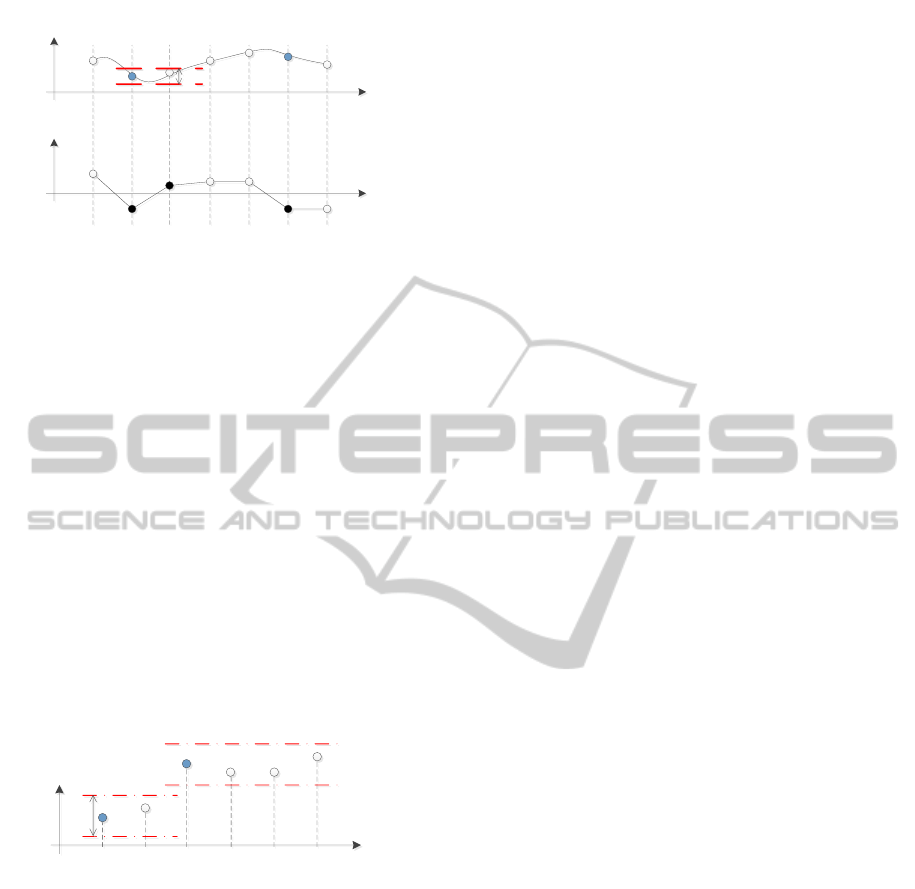
Figure 2: The anchor point is deﬁned a point with zero

velocity but for discretized points, an approximate anchor

point is obtained.

Figure 2 shows the relation of anchor points.

Somewhere between v(k) and v(k + 1) has zero ve-

locity and thus x(k + 1) is set as the anchor point,

represented as a black circle in velocity graph and

is assumed to be new reduced point represented as a

blue circle in position graph. The next v(k + 2) also

crossed zero, and thus x(k + 2) is a candidate of the

anchor point but it is within the boundary of d

min

, so

it is abandoned.

2.2 Point with Deadband

The basic idea of the deadband has been studied by

many researchers as in (Hirche et al., 2007; Hirche

and Buss, 2007). However, in this paper, previous

method is extended to adjust the reduction level from

no reduction to maximum reduction.

Position

x(k)=y

x(k+1)

x(k+2)=y

i+1

x(k+3) x(k+4)

x(k+5)

±δ

time

Figure 3: Reduction by deadband: If x(k + i) is within the

threshold, i.e., |x(k + i) − y

| ≤ δ

, it will be abandoned,

otherwise, it will set as new transmission point y

i+1

The reduction law is simple by quantization of

data with length comparison as follows:

i+1



x(k), if kx(k) − y

k ≥ δ

none, otherwise

(3)

where x(k) is the kth original data vector, y

is the

ith reduced data. Figure 3 explains the deadband ap-

proach. A blue circle represents reduced data, y

, and

white circle represents abandoned original data.

The threshold value is deﬁned as

= γd

max

(4)

The reduction level, γ is a value in the range of

0 ≤ γ ≤ 1 representing fraction of d

max

The threshold, δ

is automatically calculated by

the user adjusted reduction level γ and the max length,

max

. As shown in Eq. (3), a new reduced data y

i+1

is deﬁned if an error between the current original data

x(k) and the current reduced data y

is larger than the

given threshold, δ

. Otherwise, no data will be stored

or transmitted.

Note that, the threshold represents the maximum

quantization error between the original and reduced

data. The reduced data y

i+1

has maximum error of

, i.e., ky

i+1

− x(k)k ≤ δ

where x(k) is set of orig-

inal data between y

and y

i+1

By adjusting γ, a user can change relative reduc-

tion ratio which is related to the error range. If γ = 0,

i.e., δ

= 0, there is no error between the reduced data

and the original data, i.e., reduction is not occurred. If

γ = 1, i.e., δ

= d

max

, almost all data are vanished be-

cause d

max

is a maximum magnitude of a signal.

In the case of maximum reduction, γ = 1, it is,

however, inconvenient if no data are stored or trans-

mitted, because we don’t have any information of the

original data. To overcome this, the maximum reduc-

tion is slightly modiﬁed to represent set of data with

minimal information of the signal by using the anchor

point described in the previous section.

In summary, the proposed algorithm has three

user deﬁned parameters, the maximum critical length,

max

, the reduction level, γ, and the minimum anchor

distance, d

min

. The maximum critical length, d

max

is a

constant and is related to the mechanical speciﬁcation

of a robot system. This value is also used in restora-

tion stage. The reduction level γ is a user deﬁned rel-

ative reduction ratio which related to the quantization

error between the original data and the reduced data.

The minimum anchor distance, d

min

is a user deﬁned

value, and is mostly related to the signal properties

such as signal noise and numerical noise. The re-

duction level, and the minimum anchor distance can

be adjusted any time, even in running the algorithm.

Note that signals for the reduction are a position and

its derivative (velocity) and thus these signals should

be obtained appropriately before reduction.

3 DATA RESTORATION

WITHOUT VIOLATING

PHYSICAL LIMITS

In the previous section, motion data are reduced with

magnitude quantization. The restoration process is to

generate a trajectory satisfying the hardware system

of a target robot from randomly transmitted data in

real time.

ICINCO2014-11thInternationalConferenceonInformaticsinControl,AutomationandRobotics

362

As shown in the previous works(Hinterseer et al.,

2008), they used a zero-order-hold strategy or the lin-

ear prediction method to restore reduction data. A

zero-order-hold strategy holds a received sample un-

til a new sample arrives, and the linear prediction

method uses an average change-of-rate from the pre-

viously received samples to extrapolate current sam-

ple. All these methods and other prediction methods

always give discontinuity when a new sample arrives,

since the prediction cannot predict future motion ex-

actly. From the aspect of control, discontinuity makes

system unstable.

In addition to this discontinuity one more severe

problem not mentioned in the previous research is that

the hardware limit. The reduced data can be applied to

any robot with different hardware speciﬁcations. For

example, two robots have the same mechanical struc-

ture but their actuator limits such as acceleration, ve-

locity and position limit can be different from each

other. In this case, the reduced data should be restored

to signals that are not violating the hardware limits of

each robot.

In order to solve these problems, a convolution

interpolation is proposed to obtain continuous and

hardware-compatible motion data in real time.

3.1 Convolution Interpolation to

Generate a Trajectory

The convolution interpolation has several useful as-

pects: it can generate continuously differentiable tra-

jectories without violating physical system limits by

applying successive convolution operation; a recur-

sive form of discrete convolution can reduce compu-

tational loads drastically. In this subsection, the con-

volution interpolation to generate a trajectory shown

in (Lee et al., 2011; Lee et al., 2012) is summarized

brieﬂy.

Let us suppose that y

(t) is an non-convoluted in-

put function deﬁned in [0,t

], h(t) is a rectangular

function of unit area deﬁned in time duration [0,t

and y

(t) is the 1st output function convoluted by two

functions y

(t) and h(t). Then the convolution has

following properties:

1. The ﬁnal time t

of y

(t) is the sum of both time

durations of y

(t) and h(t), i.e., t

= t

2. The area of output y

(t) is always equal to that of

input, y

(t).

3. The maximum absolute value of y

(t) is always

less than or equal to that of y

(t). Especially, if the

input maintains a constant over the time duration

, then output reaches the input value.

(t)

1/t

(t)

1/t

(t)

1/t

(t)





(t)

n-1

(t)







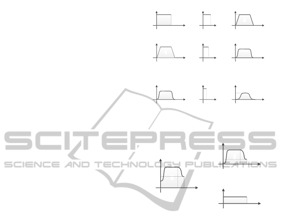
Figure 4: The effect of the convoluted trajectory with non-

zero ﬁnal condition is shown. The trajectory becomes

smoother with more convolutions.

(t)





-v

(t)





(t)





Figure 5: A general trajectory with non-zero initial and ﬁnal

velocity can be calculated by decomposing the trajectory

into non-zero initial and non-zero ﬁnal condition.

With the above properties, convolution operation

can be used for generating a trajectory as shown in

Figure 4. The initial and the ﬁnal velocity are as-

sumed zero, v

= v

= 0, and v

is the kth convoluted

velocity. S

are the area calculated with the kth convo-

lution and are equal regardless of k from the property

2. After the 1st convolution, the input y

(t) function

which is a class C

−1

function becomes a continuous

but not a differentiable function y

(t), i.e., y

(t) be-

comes a C

function. After the 2nd convolution, the

input y

(t) function becomes a function y

(t) which

has a continuous ﬁrst-derivatives, i.e., a C

function,

and so on. Consequently, by increasing the number of

convolution, we can increase the order of differentia-

bility as many as we want, and it can be represented

as y

(t) is a C

k−1

function. In convolution, the com-

pletion time is also increased from the property 1.

Figure 5 shows the case of non-zero initial and ﬁ-

nal velocity. The area S

is divided into two area:

a translated area S

with zero initial velocity and a

rectangular base area S

with the initial velocity, v

By adding two area, the entire area can be obtained,

AReal-timeMotionDataReductionandRestorationCompatiblewithRobot'sPhysicalLimits

363

= S

+ S

In order to guarantee that the resultant function

does not violate system limits, the time duration t

a unit-area function h

(t) becomes

k−1

max

for k = 1,2, ·· · ,n (5)

where v

max

denotes the system limits of kth convolu-

tion. For example, v

max

, v

max

, and v

max

denote the

maximum velocity, acceleration, jerk, respectively.

By using Eq. (5) and from property 3, we can guar-

antee the convolution interpolation does not violate

the system limits.

From Figure 5, total moving distance is repre-

sented as follows:

= S

+ S

= v

+ v

)

∑

k=1

(6)

There are two cases in using Eq. (6) with known

: 1) if v

= v

max

, then the only unknown is t

, 2) if

the ﬁnal time t

is known, then t

can be obtained from

property 1 and Eq. (5), and thus the only unknown is

. These relations can be solved as follows:

Max Velocity. If v

= v

max

, then we can arrive S

fast as possible and time t

for this can be obtained as

follows from Eq. (6)

−

+ v

)

∑

k=1

max

(7)

Known Final Time. If we know the ﬁnal time, t

go, then t

can be obtained from Property 1 as follows:

= t

−

∑

k=1

(8)

Note that t

is equal to zero or negative if given time

interval, t

is too short. This means that it is impos-

sible to reach the target with the system limits within

the given time interval. For positive t

, v

is obtained

as follows:

−

+ v

)

∑

k=1

(9)

So far convolution operation is described in the

continuous time domain, but for fast and simple cal-

culation, it can be expressed in the discrete time do-

main as follows: The convolution sum considered

with nth unit-area function, h

[k] for 0 ≤ k ≤ m

− 1

can be expressed by a recursive form as follows:

[k] =

n−1

[k] − y

n−1

[k − m

]

+ y

[k − 1] (10)

where k and m

are positive integers satisfying k =

[t/T

] and m

= [t

], respectively, with sampling

time T

and Gauss ﬂoor function [x] to denote the

largest integer not greater than x.

3.2 Continuously Restored Trajectory

with Convolution

In the previous subsection, a convolution interpola-

tion is introduced and will be used to restore the re-

duced motion data. Without loss of generality, we

only use the 1st convolution which preserves up to the

acceleration. If more hardware limits are supposed to

be satisﬁed, more order of convolution is needed, and

the relations can be obtained similarly.

Position

time

i+1

(1)

(2)

(0)

(n)

i+1

(0)

i+1

(k)

Predicted

trajectory

Original

Trajectory

Interpolated

Trajectory

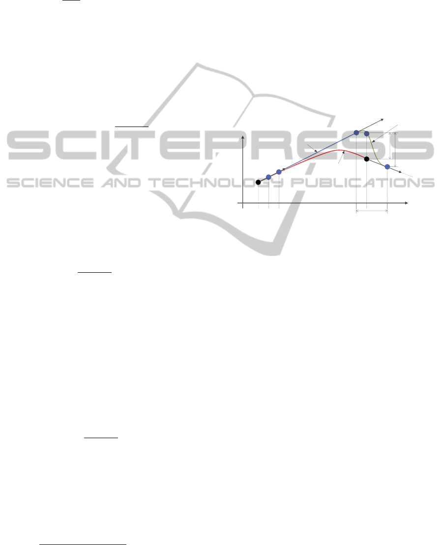
Figure 6: When a new point is arrived, there is a gap, S

, be-

tween the predicted point, r

(n) and the arrived point, y

i+1

This gap is interpolated by using the convolution method as

fast as possible without violating system limits.

In restoring data, a linear prediction is used, i.e.,

when a reduced point is composed of the point x(i)

and the velocity v(i). With these information, the re-

stored point, r

(k) becomes

(k) = v(i) · (k∆t) + x(i) (11)

where i and k are indexes for the ith transmitted data,

and kth restored data, respectively. ∆t is the sam-

pling time which may be different from the reduction

side. In the case that the velocity is not available, the

last transmitted point can used for restored data, i.e.,

(k) = x(i), and this will give more errors than the

linear prediction case.

As shown in Figure 6, the gap between the cur-

rent predicted point to the newly transmitted point is

interpolated by the convolution method as fast as pos-

sible. In the ﬁgure, the linear prediction is used with

the transmitted instantaneous velocity. It is also pos-

sible to use a zero-order-holder strategy or any other

prediction methods, but the important thing is the gap

between the current point and the newly transmitted

point.

in Figure 6 is the distance between the current

point and the newly transmitted point, but it is hard to

reach on the newly arrived point within one sampling

ICINCO2014-11thInternationalConferenceonInformaticsinControl,AutomationandRobotics

364

time in general, and thus we need more time. For the

linear prediction case as shown in Figure 6, we need

to go more distance S

calculated as follows:

= S

+ v

(12)

where v

is the transmitted ﬁnal velocity, and t

the time for reaching out to S

. The distance S

can

also be calculated as in Eq. (6) and by equating with

Eq. (12),

+ v

= v

max

+ v

)

(13)

where v

in Eq. (6) is replaced with the maximum ve-

locity, v

max

, and t

= t

from property 1. v

is the

velocity of the current point. Finally, by solving the

above equation, t

becomes

= (s

−

− v

)/(v

max

− v

) (14)

where t

= v

max

as in Eq. (5). Note that if the

linear prediction is not used, then S

= S

and thus

the term for the linear prediction v

becomes zero

in Eq. (13).

Now, we know all variables to interpolate between

the current point, r

(n), and the newly transmitted

point, y

i+1

. By applying the convolution interpola-

tion, we can connect the points smoothly and quickly

without violating the hardware limits. Note that the

error between the current point and the newly trans-

mitted point is reduced as fast as possible with the

maximum velocity and acceleration. Note also that

the signal distortion almost always exists whenever a

new point is transmitted, and it is related to the thresh-

old value, δ

4 EXPERIMENTS

In order to verify the proposed reduction/restoration

method, real motion data are obtained from a 6 DOF

arm attached on the humanoid Mahru developed by

KIST. The maximum length d

max

is set to 1m for con-

venience although the actual length is 0.72m when the

arm is unfolded straightly.

Arbitrary motions are conducted to analyze the

performance. In this paper, we only considered the

position (x,y, z) of the end-effector. Other values such

as joint angles can be considered similarly.

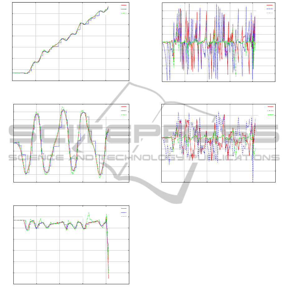
4.1 Data Reduction

The position signal has three elements (x,y, z), but for

calculating the anchor points, each signal is calculated

independently, because the anchor point represents

the stationary point with zero velocity. If all three ele-

ments are considered together as a vector, each signal

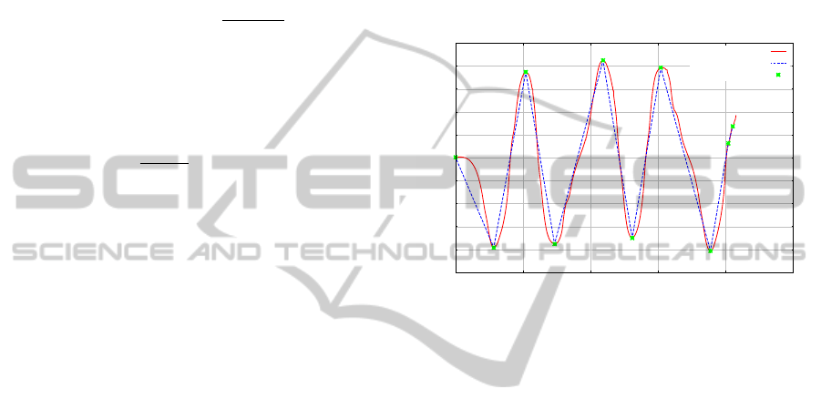
loses its shape information. Figure 7 represents the

anchor points of the y element. The anchor points,

green points in the ﬁgure, indicate points where the

direction is changed and they are the minimum num-

ber of points to present the shape of original signal as

shown in the ﬁgure with the blue line. In calculating

the anchor point, The minimum anchor distance is set

as d

min

= 0.005m. The original data has 2078 points

and the number of anchor points is 10 for y element.

0.22

0.24

0.26

0.28

0.3

0.32

0.34

0.36

0.38

0.4

0.42

0 500 1000 1500 2000 2500

distance (m)

Sampling Number

original

connected anchor point

anchor point

Figure 7: Anchor points of y element. The red line rep-

resents the original signal and discontinuous points on the

blue line represent the anchor points.

For the deadband approach, the distance is calcu-

lated with the position vector unlike the anchor point,

because relative relations of each element are impor-

tant. The blue line in Figure 8 represents the reduction

results. The reduction ratio for this case is 4.23% (88

/ 2078) with the linear prediction.

The error due to the reduction is shown in Fig-

ure 9(a). The error can be estimated by the reduction

level γ. In this case, γ = 0.01 is used and thus the

maximum error is γd

max

= 0.01m, which is valid as

shown in Figure 9(a).

4.2 Data Restoration

The green line of Figure 8 shows the restoration re-

sults with the convolution interpolation and the lin-

ear prediction. As shown in the ﬁgure, all the dis-

continuity points are connected smoothly. If more

smoothness is needed, we only need more convolu-

tions which need more delay in restoration.

The error level of the restored data shown in Fig-

ure 9(b) is similar to the reduction error shown in Fig-

ure 9(a). In most cases, the restoration error level is

equal to the reduction error, because the role of the

convolution interpolation is to connect the discontinu-

ity, i.e., it does not give additional error. However, in

AReal-timeMotionDataReductionandRestorationCompatiblewithRobot'sPhysicalLimits

365

0.1

0.2

0.3

0.4

0.5

0.6

0.7

500 1000 1500 2000 2500

Position (m)

Sample Number

original

received

linear prediction + convolution

(a) x

0.22

0.24

0.26

0.28

0.3

0.32

0.34

0.36

0.38

0.4

0.42

0 500 1000 1500 2000 2500

Position (m)

Sample Number

original

received

linear prediction + convolution

(b) y

0.51

0.52

0.53

0.54

0.55

0.56

0.57

0.58

0 500 1000 1500 2000 2500

Position (m)

Sample Number

original

received

linear prediction + convolution

Figure 8: Results of data reduction and restoration. The red

line is for the original signal, the blue line for the reduced

signal and the green line for the restored signal.

some cases, there are larger errors. This comes from

the combination of wrong prediction, numerical error,

convolution interpolation, and different hardware lim-

its. For example, the convolution interpolation gives

a different trajectory from the original one in direc-

tion change to connect points smoothly. But in most

cases, the convolution interpolation gives desired re-

sults if the hardware limits are not so poor.

-0.01

-0.008

-0.006

-0.004

-0.002

0.002

0.004

0.006

0.008

0.01

500

1000 1500 2000

2500

error (m)

Sample Number

error x

error y

error_z

(a) reduction

-0.02

-0.015

-0.01

-0.005

0.005

0.01

0.015

0 500 1000 1500 2000 2500

Error (m)

Sample Number

error_x

error_y

error_z

(b) restoration

Figure 9: Error of data reduction(a) and restoration(b). All

errors in reduction and restoration are related the reduction

level γ and the maximum critical length d

max

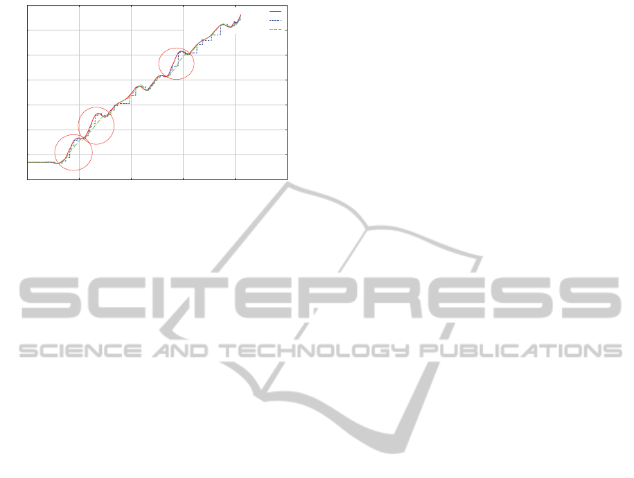
The green line in Figure 10 shows the result of the

convolution when the maximum velocity is 0.1 times

less than that of the original system. In this case, as

shown in the ﬁgure with red circles, the system cannot

follow the original signal because it has lower maxi-

mum velocity, but the restored trajectory is generated

with the maximum velocity to follow the given origi-

nal trajectory as fast as possible. The convolution in-

terpolation gives a smooth trajectory even in the case

of a low performance system, and this property is very

important for the safety aspect.

Note that the proposed method is to reduce and

restore a signal, and thus it does not have any limit

of signal type, but if a signal is nosy such as force

and acceleration, we need to choose parameters care-

fully. In addition, derivate of the signal is also needed

in reduction stage, and this magniﬁes the noise too.

Consequently, in order to improve the performance,

the relation between the parameters and signal noise

needs to be analyzed further.

ICINCO2014-11thInternationalConferenceonInformaticsinControl,AutomationandRobotics

366

0.1

0.2

0.3

0.4

0.5

0.6

0.7

0 500 1000 1500 2000 2500

Position (m)

Sample Number

original

received

linear prediction + convolution

Figure 10: Restoration results when the maximum velocity

is less than the original one. At several places enclosed by

red circles, the green line cannot follow the red line because

of the hardware limits.

5 CONCLUSIONS

In reduction and restoration of motion data, most re-

searchers focused on the reduction and not on the

restoration. However, the restoration is also impor-

tant because of the difference of hardware limits. In

the paper, we suggested a convolution based motion

data restoration method to restore data without vio-

lating the hardware limits and to generate a smooth

trajectory in real-time. In addition, we can expect

error level in reduction and restoration by using the

proposed method. With only 4.23% of the original

data, we can restore the signal with the error level

of 0.01m. The proposed method can be used in any

tele-operation and tele-presence system and for the

data storage. Especially, the proposed method is use-

ful for a poor communication environment, heteroge-

neous master-slave system, and simultaneous control

of multi-robot.

ACKNOWLEDGEMENTS

This work is supported by the KIST institutional pro-

gram (Project No. 2E24800).

REFERENCES

Hinterseer, P., Hirche, S., Chaudhuri, S., Steinbach, E., and

Buss, M. (2008). Perception-based data reduction and

transmission of haptic data in telepresence and tele-

action systems. IEEE TRANSACTIONS ON SIGNAL

PROCESSING, 56(2):588–597.

Hirche, S. and Buss, M. (2007). Transparent data reduction

in networked telepresence and teleaction systems. part

ii: Time delayed communication. Presence: Teleop-

erators Virtual Environment, 16(5):531–542.

Hirche, S., Hinterseer, P., Steinbach, E., and Buss, M.

(2007). Transparent data reduction in networked

telepresence and teleaction systems. part i: Commu-

nication without time delay. Presence: Teleoperators

Virtual Environment, 16(5):523–531.

Kron, A., Schmidt, G., Petzold, B., Zah, M. F., Hinter-

seer, P., and Steinbach, E. (2004). Disposal of ex-

plosive ordnances by use of a bimanual haptic telep-

resence system. In IEEE International Conference on

Robotics and Automation, pages 1968–1973.

Lee, G., Kim, D., and Choi, Y. (2012). Faster and smoother

trajectory generation considering physical system lim-

its under discontinuously assigned target angles. In

IEEE International Conference on Mechatronics and

Automation, pages 1196–1201, Chengdu, China.

Lee, G., Yi, B.-J., Kim, D., and Choi, Y. (2011). New

robotic motion generation using digital convolution

with physical system limitation. In IEEE Conference

on Decision and Control and European Control Con-

ference (CDC-ECC), pages 698–703, Orlando, FL,

USA.

Sakr, N., Georganas, N. D., and Zhao, J. (2010). Ex-

ploring human perception-based data reduction for

haptic communication in 6-dof telepresence systems.

In IEEE International Symposium on Haptic Audio-

Visual Environments and Games (HAVE), pages 1–6,

Phoenix, AZ.

Sakr, N., Georganas, N. D., and Zhao, J. (2011). Human

perception-based data reduction for haptic communi-

cation in six-dof telepresence systems. IEEE Trans.

on Instrumentation and Measurement, 60(11):3534–

3546.

Shahabi, C., Ortega, A., and Kolahdouzan, M. R. (2002).

A comparison of different haptic compression tech-

niques. In IEEE International Conference on Multi-

media and Expo (ICME ’02), pages 657–660.

Steinbach, E., Hirche, S., Kammerl, J., Vittorias, I., and

Chaudhari, R. (2011). Haptic data compression and

communication: A review of the challenges for telep-

resence and teleaction. IEEE SIGNAL PROCESSING

MAGAZINE, pages 87–96.

AReal-timeMotionDataReductionandRestorationCompatiblewithRobot'sPhysicalLimits

367