Keeping Intruders at Large

A Graph-theoretic Approach to Reducing the Probability of Successful Network

Intrusions

∗

Paulo Shakarian

, Damon Paulo

, Massimiliano Albanese

and Sushil Jajodia

3,4

Arizona State University, Tempe, AZ, U.S.A.

U.S. Military Academy, West Point, NY, U.S.A.

George Mason University, Fairfax, VA, U.S.A.

The MITRE Corporation, McLean, VA, U.S.A.

Keywords:

Moving Target Defense, Adversarial Modeling, Graph Theory.

Abstract:

It is well known that not all intrusions can be prevented and additional lines of defense are needed to deal with

intruders. However, most current approaches use honeynets relying on the assumption that simply attracting

intruders into honeypots would thwart the attack. In this paper, we propose a different and more realistic

approach, which aims at delaying intrusions, so as to control the probability that an intruder will reach a

certain goal within a speciﬁed amount of time. Our method relies on analyzing a graphical representation

of the computer network’s logical layout and an associated probabilistic model of the adversary’s behavior.

We then artiﬁcially modify this representation by adding “distraction clusters” – collections of interconnected

virtual machines – at key points of the network in order to increase complexity for the intruders and delay the

intrusion. We study this problem formally, showing it to be NP-hard and then provide an approximation algo-

rithm that exhibits several useful properties. Finally, we present experimental results obtained on a prototypal

implementation of the proposed framework.

1 INTRODUCTION

Despite signiﬁcant progress in the area of intrusion

prevention, it is well known that not all intrusions

can be prevented, and additional lines of defense are

needed in order to cope with attackers capable of

circumventing existing intrusion prevention systems.

However, most current approaches are based on the

use of honeypots, honeynets, and honey tokens to

lure the attacker into subsystems containing only fake

data and bogus applications. Unfortunately, these

approaches rely on the unrealistic assumption that

simply attracting an intruder into a honeypot would

thwart the attack. In this paper, we propose a totally

different and more realistic approach, which aims at

delaying an intrusion, rather than trying to stop it, so

as to control the probability that an intruder will reach

∗

This work was partially supported by the Army Re-

search Ofﬁce under award number W911NF-13-1-0421.

Paulo Shakarian and Damon Paulo were supported by the

Army Research Ofﬁce project 2GDATXR042. The work of

Sushil Jajodia was also supported by the MITRE Sponsored

Research Program.

a certain goal within a speciﬁed amount of time and

keep such probability below a given threshold.

Our approach is aligned with recent trends in cy-

ber defense research, which has seen a growing in-

terest in techniques aimed at continuously changing a

system’s attack surface in order to prevent or thwart

attacks. This approach to cyber defense is generally

referred to as Moving Target Defense (MTD) (Jajodia

et al., 2013) and encompasses techniques designed to

change one or more properties of a system in order

to present attackers with a varying attack surface

, so

that, by the time the attacker gains enough informa-

tion about the system for planning an attack, its attack

surface will be different enough to disrupt it.

In order to achieve our goal, our method relies on

analyzing a graphical representation of the computer

network’s logical layout and an associated probabilis-

tic model of the adversary’s behavior. In our model,

an adversary can penetrate a system by sequentially

gaining privileges on multiple system resources. We

Generally, the attack surface refers to system resources

that can be potentially used for an attack.

Shakarian P., Paulo D., Albanese M. and Jajodia S..

Keeping Intruders at Large - A Graph-theoretic Approach to Reducing the Probability of Successful Network Intrusions.

DOI: 10.5220/0005013800190030

In Proceedings of the 11th International Conference on Security and Cryptography (SECRYPT-2014), pages 19-30

ISBN: 978-989-758-045-1

 2014 SCITEPRESS (Science and Technology Publications, Lda.)

model the adversary as having a particular target (e.g.,

an intellectual property repository) and show how to

calculate the probability of him reaching the target in

a certain amount of time (we also discuss how our

framework can be easily generalized for multiple tar-

gets). We then modify our graphical representation

by adding “distraction clusters” – collections of inter-

connected virtual machines – at key points of the net-

work in order to reduce the probability of an intruder

reaching the target. We study this problem formally,

showing it to be NP-hard and then provide an approx-

imation algorithm that possesses several useful prop-

erties. We also describe a prototypal implementation

and present our experimental results.

Related Work. Moving Target Defense (MTD) (Ja-

jodia et al., 2013; Jajodia et al., 2011; Evans et al.,

2011) is motivated by the asymmetric costs borne by

cyber defenders. Unlike prior efforts in cyber secu-

rity, MTD does not attempt to build ﬂawless systems.

Instead, it deﬁnes mechanisms and strategies to in-

crease complexity and costs for attackers. The recent

trend of high-proﬁle cyber-incidents resulting in sig-

niﬁcant intellectual property theft (Shakarian et al.,

2013) indicates that current practical approaches may

be insufﬁcient.

MTD differs from current practical approaches

which primarily rely on three aspects: (a) attempting

to remove vulnerabilities from software at the source,

(b) patching software as rapidly as possible, and (c)

identifying attack code and infections. The ﬁrst ap-

proach is necessary but insufﬁcient because of the

complexity of software. The second approach is stan-

dard practice in large enterprises, but has proven dif-

ﬁcult to keep ahead of the threat, nor does it provide

protection against zero-day attacks. The last approach

is predicated on having a signature of malicious at-

tacks, which is not always possible.

MTD approaches aiming at selectively altering a

system’s attack surface (Manadhata and Wing, 2011)

are relatively new. In Chapter 8 of (Jajodia et al.,

2011), Huang and Ghosh present an approach based

on diverse virtual servers, each conﬁgured with a

unique software mix, producing diversiﬁed attack sur-

faces. In Chapter 9, Al-Shaer investigates an ap-

proach to enables end-hosts and network devices to

change their conﬁguration (e.g., IP addresses). In

Chapter 6, Rinard describes mechanisms to change a

system’s functionality in ways that eliminate security

vulnerabilities while leaving the system able to pro-

vide acceptable functionality. A game-theoretic ap-

proach to increase complexity for the attacker is pre-

sented in (Sweeney and Cybenko, 2012).

The efforts that are more closely related to our

work are those based on the use of honeypots. How-

ever, such approaches signiﬁcantly differ from our

work in that they aim at either capturing the at-

tacker and stopping the attack (Abbasi et al., 2012)

or collecting information about the attacker for foren-

sic purposes (Chen et al., 2013). There is also a

relatively new corpus of work on attacker-defender

models for cyber-security using game-theoretic tech-

niques: an overview is provided in (Alpcan and Baar,

2010). Work in this area related to this paper include

(Williamson et al., 2012) and (P

ıbil et al., 2012). The

work presented in (Williamson et al., 2012) is similar

to our work in that it models the adversary as moving

through a graphical structure. However, that work dif-

fers in that the defender is trying to learn about the at-

tacker’s actions for forensic analysis purposes. In this

work, we do not assume a forensic environment and

rather than trying to understand the adversary, we are

looking to delay him from obtaining access to certain

machines (e.g., intellectual property repositories). In

ıbil et al., 2012), the authors use game theoretic

techniques to create honeypots that are more likely

to deceive (and hence attract) an adversary. We view

their approach as complementary to ours, speciﬁcally

with regard to the creation of distraction clusters.

2 TECHNICAL PRELIMINARIES

In this section, we ﬁrst introduce the notion of in-

truder’s penetration network, and then provide a for-

mal statement of the problem we address in the pa-

per. Note that we model a complex system as a set

S = {s

,...,s

} of computer systems. Each system

in S is associated with a level of access obtained by

the intruder denoted by a natural number in the range

L = {0, . . . , ℓ

max

}. The level of access to a given sys-

tem changes over time, which is treated as discrete

intervals in the range 0,...,t

max

For a given system s and level ℓ, we shall use a

system-level pair (s,ℓ) to denote that the intruder cur-

rently has level of access ℓ on system s. We shall use

S to denote the set of all system-level pairs.

Deﬁnition 1

(Intruder’s penetration network (

IPN

))

Given a system S = {s

,...,s

}, the intruder’s pen-

etration network for S is a directed graph IPN =

(S,R,π,f), where S is the set of nodes representing

individual computer systems, R ⊆ S × S is a set of di-

rected edges representing relationships among those

systems. For a given s

∈ S, η

= {(s

′

) ∈ R}. We

deﬁne the conditional success probability function

π : S ×S → [0,1] as a function that, given two system-

level pairs (s,ℓ),(s

′

,ℓ

′

) returns the probability that an

intruder with access level ℓ on s will gain access level

ℓ

′

on s

′

in the next time step (provided that the attacker

SECRYPT2014-InternationalConferenceonSecurityandCryptography

Attack Source Inside Router Inside Switch

IA Switch #1 Oracle: DBSRV2

Figure 1: Sample network based on a real-world case: an

attacker targeting the Oracle server penetrates the network

exploiting a vulnerability in the Router.

selects s

′

as the next target). This function must have

the following properties:

(∀(s,s

′

)∈R)(∀ℓ>0)(π((s,0),(s

′

,ℓ))=0) (1)

(∀(s,s

′

)/∈R)(∀ℓ,ℓ

′

>0)(π((s,ℓ),(s

′

,ℓ

′

))=0) (2)

(∀ℓ

∈L )(ℓ

≤ℓ

⇒π((s,ℓ

),(s

′

,ℓ

))≤π((s,ℓ

),(s

′

,ℓ

))) (3)

We deﬁne f : S×S → ℜ as a function that provides

the “ﬁtness” of a relationship. The intuition behind

the ﬁtness f((s

,ℓ

),(s

,ℓ

)) is that it is associated with

the desirability for the attacker (who is currently on

system s

with level ℓ

) to achieve level of access ℓ

system s

. If (s

) /∈ R then f((s

,ℓ

),(s

,ℓ

)) = 0.

We note that, there are mature pieces of software

for generating the graphical structure of the IPN along

with the success probability and ﬁtness function such

as Cauldron and Lincoln Labs’ NetSpa. Additionally,

there are vulnerability databases that can aide in the

creation of an IPN as well. For instance, in NIST’s

NVD database

, impact and attack difﬁculty can map

to ﬁtness and the inverse of the probability of suc-

cess. While we are currently working with Cauldron

to generate the IPN, we do not focus on the creation of

the structure in this paper, but rather on reducing the

overall probability of success of the intruder.

We assume that if a user has no access (i.e., level 0

access) to a system s then the probability of success-

fully inﬁltrating another system s

′

from that system

is 0, which is why property 1 in Deﬁnition 1 above

is valid and necessary. Similarly, property 2 articu-

lates the fact that if no edge exists between s and s

′

then the likelihood of a successful attack on s

′

origi-

nating from s is also 0. Finally, property 3 deﬁnes the

intuitive assumption that if an attacker can complete

an attack with a certain probability of success then

if he conducts the same attack with a higher level of

permissions on the original system his probability of

success must be at least the same as it was in the orig-

inal attack.

Example 2.1. Consider the simple network displayed

in Fig. 1 which represents a subset of a real world

http://nvd.nist.gov/

network we examined. In this network a user can

have one of two levels of access on each system; he

can have guest privileges (ℓ

= 1) or root privileges

(ℓ

= 2). The attacker begins with root privileges

on his personal device (s

,2). The network is dis-

played in full in Fig. 2 where nodes represent system-

level pairs and edges represent logical connections

between them. All transitions between system-level

pairs will either involve transitioning to a new system

or to a higher level on the current system. Edges rep-

resenting gaining higher access on the current sys-

tem are red and bold in Fig. 2. Given two system-

level pairs ((s

,ℓ

),(s

,ℓ

)), the ﬁtness of the relation-

ship

between them (f((s

,ℓ

),(s

,ℓ

))) is shown on

the edge between them as f, and the conditional suc-

cess probability function (π((s

,ℓ

),(s

,ℓ

))) is shown

as π. For example, in the sample network, when the

attacker begins with root access on his personal com-

puter (s

,2) he can gain guest privileges on the inside

router (s

,1) with a ﬁtness of 1 and a probability of

success of 0.8. For ease of reading, for all system-

level pairs where f((s

,ℓ

),(s

,ℓ

)) = 0 the edge is not

displayed. The probability of a successful attack oc-

curring is the product of the probability that the at-

tack succeeds and the probability that the attack is

selected by the intruder. In our sample network, then,

when the intruder has guest privileges on the inside

router (s

,1) his probability of successfully gaining

root access on that router (s

,2) in the next time step

1+1

× 0.6 = 0.3.

Penetration Sequence. A penetration se-

quence is simply a sequence of system-level

pairs ⟨(s

,ℓ

),...,(s

,ℓ

)⟩ such that for each

a = (s

,ℓ

),b = (s

i+1

,ℓ

i+1

) in the sequence we have

r = (s

i+1

) ∈ R , π(a,b), f (a, b) > 0. For a sequence

σ we shall denote the number of system-level

pairs with the notation |σ|. For a given sequence

σ, let σ

be the sub-sequence of σ consisting of

the ﬁrst m − 1 system-level pairs in σ. For a se-

quence σ = ⟨(s

,ℓ

),...,(s

,ℓ

)⟩, curSys(σ) = s

curLvl(σ) = ℓ

and cur(σ) = (s

,ℓ

). We use the

notation next(σ) to denote the set of system-level

pairs that could occur next in the sequence. Formally:

next(σ)={(s,ℓ)∈S | ℓ>0∧(curSys(σ),s)∈R∧

̸∃ℓ

′

≥ℓ s.t. (s,ℓ

′

)∈σ} (4)

We note that in this particular example we have set the

ﬁtness values to all be one. Note that this is just one way

to specify a ﬁtness function - perhaps in the case with no

information about desirability of a system (i.e. akin to using

uniform priors). All of our results and algorithms are much

more general and allow for arbitrary ﬁtness values.

KeepingIntrudersatLarge-AGraph-theoreticApproachtoReducingtheProbabilityofSuccessfulNetworkIntrusions

Attack

Origin

Inside

Router

Inside

Router

Inside

Switch

f = 1, π = 0.8

IA Switch

f = 1, π = 0.8

f = 1, π = 0.7

f = 1, π = 0.6

f = 1, π = 0.3

f =1, π = 0.8

Oracle:

DBSRV2

Inside

Switch

Oracle:

DBSRV2

f = 1, π = 0.7

Figure 2: The sample network. Nodes are system-level pairs.

Example 2.2. Fig. 3 depicts all ﬁve possible pene-

tration sequences by which the attacker can gain root

access to the Oracle: DBSRV2 (s

,2) in our sample

network in ﬁve time steps or fewer. The penetration

sequences are labeled as σ

through σ

Model of the Intruder’s Actions. Now, we shall de-

scribe our model. Consider an attacker who has inﬁl-

trated through a sequence of systems speciﬁed by σ.

If the penetration is to continue, the intruder must se-

lect a system-level pair from next(σ). The intruder

selects exactly one system-level pair (s, ℓ) with the

following probability:

f(cur(σ), (s, ℓ))

∑

′

,ℓ

′

)∈next(σ)

f(cur(σ), (s

′

,ℓ

′

))

(5)

Hence, the probability of selection is proportional

to the relative ﬁtness of (s, ℓ) compared to the other

options for the attacker. This aligns with our idea of

ﬁtness: an intruder will attempt to gain access to sys-

tems that are more “ﬁt” with respect to his expertise,

available tools, desirability of the next system, etc.

Note that this probability of selection is not tied to

the intruder’s probability of success. In fact, we con-

sider the two as independent. Hence, the probability

that an intruder selects and successfully reaches (s,ℓ)

can be expressed as follows:

f(cur(σ), (s, ℓ))π(cur(σ),(s,ℓ))

∑

′

,ℓ

′

)∈next(σ)

f(cur(σ), (s

′

,ℓ

′

))

(6)

Hence, given that the attacker starts at a certain

(s,ℓ), we can compute the sequence probability or

probability of taking sequence σ (provided that σ

starts at (s, ℓ) – this probability would be zero oth-

erwise).

|σ|−2

∏

i=0

f(cur(σ

),cur(σ

i+1

))π(cur(σ

),cur(σ

i+1

))

∑

(s,ℓ)∈next(σ

)

f(cur(σ

),(s,ℓ))

(7)

Hence, for a given initial (s,ℓ) and ending (s

′

,ℓ

′

and length t + 1, we can compute the probability of

starting at (s,ℓ) and ending at (s

′

,ℓ

′

) in t time-steps or

less by taking the sum of the sequence probabilities

for all valid sequences that meet that criterion. For-

mally, we shall refer to this as the penetration prob-

ability and for a given IPN,t,(s,ℓ),(s

′

,ℓ

′

) we shall de-

note this probability as Pen

IPN

((s,ℓ),(s

′

,ℓ

′

)). Intuitively,

Pen

IPN

((s,ℓ),(s

′

,ℓ

′

)) is the probability that an attacker at

system s with level of access ℓ reaches system s

′

with

level of access ℓ

′

or greater in t time steps or less.

Example 2.3. The probability of the attacker suc-

cessfully gaining access to (s

,2) in ﬁve time steps

or fewer is the sum of the probabilities of each of

the ﬁve possible penetration sequences depicted in

Fig. 3. For each penetration sequence σ

the prob-

ability of the attacker successfully gaining access to

,2) through that particular sequence is p

. For the

sample network: p

= 0.023, p

= 0.021, p

= 0.021,

= 0.004, p

= 0.016. Thus, the total probability of

a successful attack occurring on system 5 at level 2 in

three time steps or fewer is Pen

IPN

,2) = 0.085.

3 DISTRACTION CHAINS AND

CLUSTERS

We now introduce the idea of a distraction chain. A

distraction chain is simply a sequence of decoy sys-

tems that we wish to entice an adversary to explore to

distract him from the real systems of the network. In

order to entice the adversary to explore a distraction

chain, we propose adding one-way distraction clus-

ters to S. Hence, the adversary enters such a distrac-

tion cluster and is delayed from returning to the ac-

tual network for a number of time steps proportional

to the size of the cluster. Ideally, a distraction clus-

ter would be large enough to delay the attacker for

a long time; however, larger distraction clusters will

obviously require more resources to construct. Dis-

traction clusters differ from honeypots because they

do not prevent intruders from reaching other portions

of the network, thus minimizing the risk of the in-

truder realizing that he is trapped. Again, the goal

of a honeypot is to prevent an attacker from complet-

ing his attack by trapping him under the assumption

SECRYPT2014-InternationalConferenceonSecurityandCryptography

Attack

Origin

Inside

Router

IA Switch

Oracle:

DBSRV2

Inside

Switch

Oracle:

DBSRV2

Attack

Origin

Inside

Router

IA Switch

Oracle:

DBSRV2

Inside

Switch

Attack

Origin

Inside

Router

IA Switch

Oracle:

DBSRV2

Inside

Switch

IA Switch

Attack

Origin

Inside

Router

IA Switch

Oracle:

DBSRV2

Inside

Switch

Inside

Switch

Attack

Origin

Inside

Router

IA Switch

Oracle:

DBSRV2

Inside

Switch

Inside

Router

0.8

0.7

0.35 0.233 0.35

0.233 0.35

0.35

0.233

0.45

0.267

0.1 0.4

0.35

0.35 0.8 0.3

= 0.023

= 0.021

= 0.004

= 0.016

Figure 3: All possible penetration sequences with ﬁve time steps or fewer.

that once he is trapped he will not leave it, while the

goal of a distraction cluster is – more realistically –

to delay the attacker in order to reduce the probabil-

ity that he will successfully complete his attack in a

given amount of time.

Clearly, a valid distraction cluster would be con-

nected to the rest of the system through a one-way

connection and the cluster must be created in a man-

ner where there is at least one (preferably many) dis-

traction chain of the necessary length (based on an ex-

pected limit of time we expect the intruder to remain

in the network before discovery).

For now we shall leave the creation of distraction

clusters to future work (e.g., the work of (P

ıbil et al.,

2012) may provide some initial insight into this prob-

lem) and instead focus on the problem of adding dis-

traction clusters to a system. The conﬁguration of the

ﬁrst system of a distraction cluster will be a key ele-

ment in setting up a distraction chain. In particular,

the open ports, patch level, installed software, operat-

ing system version, and other vulnerabilities present

on that lead system, as well as any references of that

system found elsewhere on the network will dictate

how “ﬁt” an attacker will determine such a system

to be and the probability of success he will have in

entering into the distraction chain. Note that the ﬁt-

ness of this ﬁrst system cannot be arbitrarily high and

should be considered based on a realistic assessment

of why the attacker would select such a system. Fur-

ther, the probability of an adversary obtaining privi-

leges on such a system should be set in such a way

where it is not overly simple for the intruder to gain

access - or he might suspect it is a decoy. Addition-

ally, the last system in the distraction cluster must be

conﬁgured in a way to reconnect it to the actual net-

work.

Throughout the paper, we will consider a set of

conﬁgurations available to the defender denoted CFG.

For instance, CFG may consist of a predetermined set

of virtual machine images available to the security

team. In addition we will consider a set of potential

distraction clusters denoted CL. For each cl ∈ CL

there exists value t

∈ N, a natural number equal to

the minimum number of time steps elapsed before

an attacker is able to leave the cluster and return

to the network. For each cfg ∈ CFG, for the lead

and last systems in the distraction cluster (resp.

dc1

, s

dc2

) there are associated conditional prob-

abilities (resp. π

cfg,cl

: S × {(s

dc1

,ℓ)} → [0,1],

cfg,cl

: {(s

dc2

,ℓ)} × S → [0,1]) and ﬁtness

function (resp. f

cfg,cl

: S × {(s

dc1

,ℓ)} → ℜ,

cfg,cl

: {(s

dc2

,ℓ)} × S → ℜ). These functions

are based on the software installed on and the vul-

nerabilities present in that particular conﬁguration.

Hence, once a distraction cluster is added it contains

a lead system conﬁgured with conﬁguration cfg.

The resulting IPN formed with the addition of

distraction cluster includes conditional probability

and ﬁtness functions that are the concatenation of

π,π

cfg,cl

and f,f

cfg,cl

respectively. Additionally, for

each s ∈ S we add (s,s

dc1

) to R where there exists

s,ℓ where ℓ > 0 s.t. π

cfg,cl

((s,ℓ),(s

dc1

,1)) > 0

and f

cfg,cl

((s,ℓ),(s

dc1

,1)) > 0 and we add

dc2

,s) to R where there exists s,ℓ where

ℓ > 0 s.t. π

cfg,cl

((s

dc2

,1),(s,ℓ)) > 0 and

cfg,cl

((s

dc2

,1),(s,ℓ)) > 0. In other words, a

logical connection is formed from all systems in

S for which, if connected to s

dc1

or s

dc2

there is a

non-zero probability that the intruder can gain a level

of access greater than ℓ = 0. We can easily restrict

which relationship are added by modifying the f

cfg,cl

functions. For a given IPN, set of distraction clusters,

and set of conﬁguration-cluster pairs PCP ⊆ CFG × CL,

we will use the notation IPN ∪ PCP to denote the

concatenation of the intrusion penetration network

and the set of conﬁguration-cluster pairs.

KeepingIntrudersatLarge-AGraph-theoreticApproachtoReducingtheProbabilityofSuccessfulNetworkIntrusions

Adding Distraction Clusters. We now have the

pieces we need to introduce the formal deﬁnition of

our problem.

Deﬁnition 2 (Cluster Addition Problem). Given IPN

(S,R,π,f), systems s,s

′

∈ S, access levels ℓ

,ℓ

′

∈ L ,

set of potential distraction clusters CL, set of conﬁgu-

rations CFG, natural number k, real number x ∈ [0,1],

and time-limit t, ﬁnd PCP ⊆ CFG × CL s.t. |PCP| ≤ k and

Pen

IPN

((s,ℓ),(s

′

,ℓ

′

)) − Pen

IPN∪PCP

((s,ℓ),(s

′

,ℓ

′

)) > x.

Example 3.1. Following along with our sample net-

work, the set of conﬁgurations, CFG, displayed in

Fig. 4, and with k = 2, t = 5, x = 0.05, and CL = {cl}

(with t

= 6) we ﬁnd that PCP = {(cfg

,cl),(cfg

,cl)}

is a solution to the Chain Addition Problem because

Pen

IPN

,2) − Pen

IPN∪PCP

,2) = 0.063 > 0.05 = x

The modiﬁed IPN is displayed in Fig. 5.

Unfortunately, this problem is difﬁcult to solve ex-

actly by the following result (the proof is provided in

the appendix).

Theorem 1. The Cluster Addition Problem is NP-

hard and the associated decision problem is NP-

Complete when the number of sequences from (s,ℓ)

to (s

′

,ℓ

′

) is a polynomial in the number of nodes in

the intruder penetration network.

For a given instance of the Cluster Addition

Problem, for a given PCP ⊆ CFG × CL let orc(PCP) =

Pen

IPN

((s,ℓ),(s

′

,ℓ

′

)) − Pen

IPN∪PCP

((s,ℓ),(s

′

,ℓ

′

)). In the opti-

mization version of this problem, this is the quan-

tity we attempt to optimize. Unfortunately, as a by-

product of Theorem 1 and the results of (Feige, 1998)

(Theorem 5.3), there are limits to the approximation

we can be guaranteed to ﬁnd in polynomial time.

Theorem 2. With a cardinality constraint, ﬁnding set

PCP s.t. orc(PCP) cannot be approximated in PTIME

within a ratio of

e−1

+ ε for some ε > 0 (where e is

the base of the natural log) unless P=NP.

However, orc does have some useful properties.

Lemma 1 (Monotonicity). For PCP

′

⊆ PCP ⊆ CFG ×CL,

orc(PCP

′

) ≤ orc(PCP).

Lemma 2 (Submodularity). For PCP

′

⊆ PCP ⊆ CFG ×

CL and pc = (cfg, cl) /∈ PCP we have:

orc(PCP ∪{pc})−orc(PCP) ≤ orc(PCP

′

∪{pc})−orc(PCP

′

)

4 ALGORITHMS

Greedy Approach. Now we introduce our greedy

heuristic for the Chain Addition Problem.

Algorithm 1: GREEDY CLUSTER.

Require: Systems s,s

′

, access levels ℓ

,ℓ

′

, set of distrac-

tion chains CL, set of protocols CFG, natural number k

and time limit t

Ensure: Subset PCP ⊆ CFG × CL

1: PCP =

2: while |PCP| ≤ k do

3: curBest = null, curBestScore = 0

4: for (cfg, cl) ∈ (CFG × CL) − PCP do

5: curScore = orc(PCP ∪ {(cfg,cl)}) − orc(PCP)

6: if curScore ≥ curBestScore then

7: curBest = (cfg,cl)

8: curBestScore = curScore

9: end if

10: end for

11: PCP = PCP ∪ {curBest}

12: end while

13: return PCP.

Example 4.1. When run on our sample net-

work, GREEDY CLUSTER selects (cfg

,cl) in the

ﬁrst iteration of the loop at line 4, lowering

Pen

IPN∪PCP

,2) from 0.085 to 0.037. In the next

iteration GREEDY CLUSTER selects (cfg

,cl), low-

ering Pen

IPN∪PCP

,2) from 0.037 to 0.022. At this

point, since |PCP| = 2 = k, GREEDY CLUSTER re-

turns PCP = {(cfg

,cl),(cfg

,cl)}, a solution to the

Chain Addition Problem under our given constraints.

Though simple, GREEDY CLUSTER, can provide

the best approximation guarantee unless P=NP under

the condition that orc can be solved in PTIME. Con-

sider the following theorem.

Theorem 3. GREEDY CLUSTER provides the best

PTIME approximation of orc unless P=NP if orc can

be solved in PTIME.

However, the condition on solving orc in PTIME

may be difﬁcult to obtain in the case of a very gen-

eral IPN. Though we leave the exact computation of

this function as an open problem, we note that the

straight-forward approach for computation would im-

ply the need to enumerate all sequences from (s,ℓ)

to (s

′

,ℓ

′

) - which can equal the number of t-sized (or

smaller) permutations of the elements of S - a quan-

tity that is not polynomial in the size of IPN. Hence,

a method to approximate orc is required in practice.

Our intuition is that the expensive computation of the

penetration probability can be approximated by sum-

ming up the sequence probabilities of the most prob-

able sequences from (s, ℓ) to (s

′

,ℓ

′

). The intuition of

approximating the probability of a path between two

nodes in a network (given a diffusion model) based on

high-probability path computation was introduced in

(Chen et al., 2010) where it was applied to the maxi-

mum inﬂuence problem. However, our approach dif-

fers in that (Chen et al., 2010) only considered the

SECRYPT2014-InternationalConferenceonSecurityandCryptography

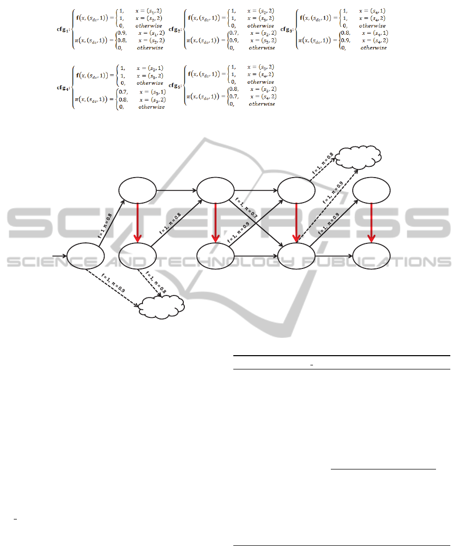
Figure 4: The set CFG of possible conﬁgurations available to the defender.

Attack

Origin

Inside

Router

Inside

Router

Inside

Switch

f = 1, π = 0.8

IA Switch

f = 1, π = 0.8

f = 1, π = 0.7

f = 1, π = 0.6

f = 1, π = 0.3

f =1, π = 0.8

Oracle:

DBSRV2

Inside

Switch

Oracle:

DBSRV2

f = 1, π = 0.7

cfg

Figure 5: The updated network with PCP added.

most probable path, as we consider a set of most prob-

able paths. Our intuition in doing so stems from the

fact that alternate paths can contribute signiﬁcantly to

the probability speciﬁed by Pen

IPN

((s,ℓ),(s

′

,ℓ

′

)).

Computing orc. Next, we introduce a simple

sampling-based method that randomly generates se-

quences from (s, ℓ) to (s

′

,ℓ

′

) of the required length.

These sequences are generated with a probability

proportional to their sequence probability, hence the

computation of orc based on these samples is biased

toward the set of most-probable sequences from (s, ℓ)

to (s

′

,ℓ

′

), which we believe will provide a close

approximation to orc. Our pre-processing method,

ORC SAM below generates a set of sequences that

the attacker could potentially take. Using the se-

quences from SEQ, we can then calculate the penetra-

tion probability (Pen

IPN

((s,ℓ),(s

′

,ℓ

′

))) by summing over

the probabilities over the sequences in SEQ as op-

posed to summing over all sequences (a potentially

exponential number).

Extensions. Our approach is easily generalizable for

studying other problems related to Cluster-Addition.

For instance, suppose an intruder initiates his inﬁltra-

tion from one of a set of systems chosen based on a

Algorithm 2: ORC SAM.

Require: Systems s, s

′

, access levels ℓ

,ℓ

′

, natural num-

bers t, maxIters

Ensure: Set of sequences SEQ

1: curIters = 0, SEQ =

2: while curIters < maxIters do

3: (s

,ℓ

) = (s, ℓ

), curSeq = ⟨(s, ℓ

)⟩, curLth = 0

4: while curLth < t and (s

,ℓ

) ̸= (s

′

,ℓ

′

) do

5: Select (s

′

,ℓ

′

) from the set (η

×L ) − curSeq with

a probability of

f((s

,ℓ

),(s

′

,ℓ

′

))π((s

,ℓ

),(s

′

,ℓ

′

))

∑

,ℓ

)∈(η

×L )−curSeq

f((s

,ℓ

),(s

,ℓ

))

6: curSeq = curSeq ∪ {(s

′

,ℓ

′

)}

7: end while

8: If (s

′

,ℓ

′

) = (s

′

,ℓ

′

) then SEQ = SEQ ∪ {curSeq}

9: curIters+ = 1

10: end while

11: Return SEQ

probability distribution. We can encode this problem

in Chain-Addition by adding a dummy system to the

penetration network and establishing relationships to

each of the potential initial systems in the set. The

ﬁtness and conditional probability functions can then

be set up in a manner to reﬂect the probability distri-

bution over the set of potential initial systems. Note

KeepingIntrudersatLarge-AGraph-theoreticApproachtoReducingtheProbabilityofSuccessfulNetworkIntrusions

that this problem would still maintain the same math-

ematical properties and guarantees of our already de-

scribed method to solve the Cluster-Addition prob-

lem. Another related problem that can be solved us-

ing our methods (again with only minor modiﬁcation)

is to minimize the expected number of compromised

systems in a set of potential targets. As the expected

number of systems would simply be the sum of the

penetration probability for each of those machines, a

simple modiﬁcation to Line 5 of GREEDY CLUSTER

would allow us to represent this problem, in this case

instead of examining orc we would examine the sum

of the value for orc returned for paths going to each of

the potential targets. Note that by the fact that posi-

tive linear combinations of submodular functions are

also submodular, we are able to retain our theoretical

guarantees here as well.

5 EXPERIMENTAL RESULTS

We conducted several experiments in order to test the

effectiveness of our algorithm under several circum-

stances. As explained in the preceding running ex-

ample we tested our algorithm on a small network

derived from a real network. As shown, by adding

two distraction clusters to that network we were able

to reduce the probability of a successful attack from

8.5% to 2.2%, an almost 75% reduction. While this

result shows relevance to a real-world network and

displays the algorithm on an easily understood scale,

we also wanted to test the scalability of our algorithm

by experimenting on larger networks. Due to the dif-

ﬁculty of obtaining large datasets for conducting re-

search in cyber security we generated random graphs

that resembled the network topology of the types of

penetration networks we wish to examine, allowing

us to test the scalability of our algorithm. To do this

we generated networks which were divided into lay-

ers, meaning that each system is only connected to

other systems in its own layer or to systems in the

next layer. This is important because it means that in

a network with

layers, the shortest path between the

source of the attack and the target is n − 1. We did

this because it mimics the topology of the real-world

networks we wished to replicate in our experiments.

It provides structure to our networks so that the sim-

ulated attackers will have to gain access to systems

across a series of layers before gaining access to a

system from which they can access their target. For

all of our experiments we assumed that π = 1. We

did this because it makes it easier to see and under-

stand the relationship between the lower and upper

bounds of the penetration probability. This does not

compromise the value of our results because adding

distraction clusters to a network only effects the rela-

tive ﬁtness of an attack, so the probability of success

for any one attack does not inﬂuence our results.

The ﬁrst test we ran sought to measure the effec-

tiveness of the ORC SAM sampling algorithm by test-

ing against the value of t—the maximum length of

a penetration sequence—and the number of iterations

conducted in the sampling algorithm (ORC SAM). We

found—as would be expected—that the number of it-

erations required for the most accurate possible result

increases as t increases and as the number of system-

level pairs (nodes) in the network increases. We ran

our tests on randomly generated networks with 50 and

100 systems each with 2 levels per system. Figs. 6, 7,

and 8 display the results of this test. Fig. 6 shows that,

as t increases, the number of iterations of ORC SAM

required to get an accurate prediction of the penetra-

tion probability increases. For high values of t, with

a relatively small number of iterations, the difference

between the upper and lower bounds of the test is very

large. This effect is displayed more clearly in Fig. 7

in which this difference is graphed for each value of

t against the number of iterations. Finally, Fig. 8 dis-

plays the time in seconds that each individual test took

to run.

One important factor when implementing distrac-

tion clusters is determining the location in the net-

work in which to place them. The initial instinct may

be that the goal should be to distract the attacker early

in his pursuit and thus the clusters should be placed

close to the source of the attack; however, this has

little effect on the resulting decrease in penetration

probability. We conducted experiments on the same

two networks from the previous test in which we ran-

domly generated a cluster and connected it to 10 sys-

tems in a given layer for each layer in the system

(other than the ﬁrst and last layers which only have

one system each—the source and the target, respec-

tively). We then measured the changes in penetration

probability that occurred as a result. For each network

we conducted 10 trials. Our results showed little ev-

idence that the proximity to the source of the attack

matters and instead suggest that the size of the layer

is the more inﬂuential variable. Clusters with con-

ﬁgurations that connected them to systems in a layer

with a relatively small number of systems showed a

larger decrease in the penetration probability. In ad-

dition to being suggested by our evidence, this also

makes intuitive sense because providing the attacker

a distraction in a layer with fewer systems means that

more of his options will lead into the distraction clus-

ter rather than allowing him to progress forward with

his attack.

SECRYPT2014-InternationalConferenceonSecurityandCryptography

0.1

0.2

0.3

0.4

0.5

0.6

0.7

0.8

0.9

5 15 25 35 45

Penetration Probability Bounds

Iterations (thousands)

t = 6 t = 7 t = 8 t = 9 t = 10 t = 11 t = 12

(a) Network with 50 systems.

0.1

0.2

0.3

0.4

0.5

0.6

0.7

0.8

0.9

10 30 50 70 90

Penetration Probability Bounds

Iterations (thousands)

t = 7 t = 8 t = 9 t = 10 t = 11

(b) Network with 100 systems.

Figure 6: Upper and lower bounds of the predicted penetration probability vs. number of iterations of ORC SAM, for different

values of t.

0.1

0.2

0.3

0.4

0.5

0.6

0.7

0.8

0.9

5 15 25 35 45

Penetration Probability Range

Iterations (thousands)

t = 6 t = 7 t = 8 t = 9 t = 10 t = 11 t = 12

(a) Network with 50 systems.

0.1

0.2

0.3

0.4

0.5

0.6

0.7

0.8

0.9

10 30 50 70 90

Penetration Probability Range

Iterations (thousands)

t = 7 t = 8 t = 9 t = 10 t = 11

(b) Network with 100 systems.

Figure 7: Difference between upper and lower bounds of the predicted penetration probability vs. number of iterations of

ORC SAM, for different values of t.

0 10 20 30 40 50

Execution Time (s)

Iterations (thousands)

t = 6 t = 7 t = 8 t = 9 t = 10 t = 11 t = 12

(a) Network with 50 systems.

100

150

200

250

300

350

0 20 40 60 80 100

Execution Time (s)

Iterations

t = 7 t = 8 t = 9 t = 10 t = 11

(b) Network with 100 systems.

Figure 8: Execution time vs. number of iterations of ORC SAM, for different values of t.

R² = 0.9437

0.1

0.12

0.14

0.16

0.18

0.2

0.22

0.24

5 7 9 11 13

Penetration Probability

Number of Systems in Layer

Lower Bound Linear (Lower Bound)

(a) Network with 50 systems.

R² = 0.9206

R² = 0.8286

0.015

0.018

0.021

0.024

0.027

0.030

0 5 10 15 20

Penetration Probability

Number of Systems in Layer

Lower Bound Upper Bound Linear (Lower Bound) Linear (Upper Bound)

(b) Network with 100 systems.

Figure 9: Correlation between the number of systems in a layer and the penetration probability when the distraction cluster

was conﬁgured to systems in that layers (note that for the network with 50 systems, the bounds nearly matched and only the

lower is displayed).

KeepingIntrudersatLarge-AGraph-theoreticApproachtoReducingtheProbabilityofSuccessfulNetworkIntrusions

0.05

0.1

0.15

0.2

0.25

0.3

5 15 25 35 45

Penetration Probability

Iterations (thousands)

Without DC With DC

(a) Network with 50 systems, t = 7.

0.1

0.2

0.3

0.4

0.5

0.6

5 15 25 35 45

Penetration Probability

Iterations (thousands)

Without DC With DC

(b) Network with 50 systems, t = 8.

0.1

0.2

0.3

0.4

0.5

0.6

0.7

0.8

0.9

5 15 25 35 45

Penetration Probability

Iterations (thousands)

Without DC With DC

0.01

0.02

0.03

0.04

0.05

0.06

10 30 50 70 90

Penetration Probability

Iterations (thousands)

Without DC With DC

(d) Network with 100 systems, t = 7.

0.1

0.2

0.3

0.4

0.5

0.6

10 30 50 70 90

Penetration Probability

Iterations (thousands)

Without DC With DC

(e) Network with 100 systems, t = 8.

0.1

0.2

0.3

0.4

0.5

0.6

0.7

0.8

0.9

10 30 50 70 90

Penetration Probability

Iterations (thousands)

Without DC With DC

(f) Network with 100 systems, t = 9.

Figure 10: Penetration probabilities before and after adding the cluster chosen by GREEDY CLUSTER.

Fig. 9 shows the results from the tests. The y-axis

represents the average penetration probability with

the conﬁguration added to the layer while the x-axis

represents the number of systems in the layer. The

dotted line shows the result of the linear regression

which shows a linear relationship between the two

variables. While we show a linear regression the rela-

tionship is not exactly linear as the effect is lessened

as the layers become larger. Note that the average

percent decrease in penetration probability when clus-

ters were added to the network with 50 systems was

20.7% while the average when they were added to the

larger network was only 6.4%. We hope to do further

testing in the future to identify other variables that af-

fect the outcome. In addition to investigating the ideal

location for placing a cluster we also examined the

effects of the number of iterations of ORC SAM that

are run on the results of the test. These results are

shown in Fig. 10. As explained earlier, ORC SAM is

a heuristic that generates a random sample of possi-

ble paths between the source and target. To test this

we ran GREEDY CLUSTER with varying numbers of

iterations run on ORC SAM. We generated ten possi-

ble conﬁgurations for GREEDY CLUSTER to choose

from and assigned it to choose the optimal conﬁgu-

ration. We ran the test on both networks with itera-

tions of ORC SAM ranging from 5,000 to 50,000 in

increments of 5,000 on the smaller network and from

10,000 to 100,000 in increments of 10,000 on the

larger one. We ran this test with the values of t—the

maximum length of a penetration sequence—set to 7,

8, and 9 for three different tests on both networks.

We found that regardless of the number of iterations

run or the value of t, GREEDY CLUSTER selected the

same conﬁguration and there was a small difference

between the percent decrease in penetration probabil-

ities after the clusters were added to the network. This

suggests that accurate predictions about the effects of

a cluster on a network can be made without sampling

all possible paths from the source to the target. Ad-

ditionally, as stated earlier, it suggests that seeking to

reduce the probability of the attack being reached in

the shortest number of steps will also help reduce the

probability of paths of greater lengths.

6 CONCLUSIONS

Despite signiﬁcant progress in the area of intrusion

prevention, it is well known that not all intrusions

can be prevented, and additional lines of defense are

needed in order to cope with attackers capable of cir-

cumventing existing intrusion prevention systems.

In this paper, we proposed a novel approach to in-

trusion prevention that aims at delaying an intrusion,

rather than trying to stop it, so as to control the proba-

bility that an intruder will reach a certain goal within

a speciﬁed amount of time. In the future, we plan to

do more experiments to better understand the factors

that inﬂuence the ideal location of distraction clus-

SECRYPT2014-InternationalConferenceonSecurityandCryptography

ters and to determine the relationship between pen-

etration probability, iterations of ORC SAM, and the

selection of conﬁgurations for adding distraction clus-

ters as well as investigate the impact of the length of

distraction clusters on the network and the location of

the point at which the distraction clusters reconnect to

the network.

REFERENCES

Abbasi, F., Harris, R., Moretti, G., Haider, A., and An-

war, N. (2012). Classiﬁcation of malicious network

streams using honeynets. In Global Communications

Conference (GLOBECOM), pages 891–897.

Alpcan, T. and Baar, T. (2010). Network Security: A Deci-

sion and Game-Theoretic Approach. Cambridge Uni-

versity Press, New York, NY, USA, 1st edition.

Chen, C.-M., Cheng, S.-T., and Zeng, R.-Y. (2013). A

proactive approach to intrusion detection and malware

collection. Security and Communication Networks,

6(7):844–853.

Chen, W., Wang, C., and Wang, Y. (2010). Scalable in-

ﬂuence maximization for prevalent viral marketing in

large-scale social networks. In Proceedings of the 16th

ACM SIGKDD international conference on Knowl-

edge discovery and data mining, pages 1029–1038.

Evans, D., Nguyen-Tuong, A., and Knight, J. C. (2011).

Moving Target Defense: Creating Asymmetric Un-

certainty for Cyber Threats, chapter Effectiveness of

Moving Target Defenses, pages 29–48. Springer.

Feige, U. (1998). A threshold of ln n for approximating set

cover. J. ACM, 45(4):634–652.

Jajodia, S., Ghosh, A. K., Subrahmanian, V. S., Swarup, V.,

Wang, C., and Wang, X. S., editors (2013). Moving

Target Defense II: Application of Game Theory and

Adversarial Modeling, volume 100 of Advances in In-

formation Security. Springer, 1st edition.

Jajodia, S., Ghosh, A. K., Swarup, V., Wang, C., and Wang,

X. S., editors (2011). Moving Target Defense: Cre-

ating Asymmetric Uncertainty for Cyber Threats, vol-

ume 54 of Advances in Information Security. Springer.

Manadhata, P. K. and Wing, J. M. (2011). An attack surface

metric. IEEE Transactions on Software Engineering,

37(3):371–386.

Nemhauser, G. L., Wolsey, L. A., and Fisher, M. (1978).

An analysis of approximations for maximizing sub-

modular set functionsi. Mathematical Programming,

14(1):265–294.

ıbil, R., Lis

y, V., Kiekintveld, C., Bosansk

y, B., and Pe-

choucek, M. (2012). Game theoretic model of strate-

gic honeypot selection in computer networks. In

GameSec, pages 201–220.

Shakarian, P., Shakarian, J., and Ruef, A. (2013). Introduc-

tion to Cyber-Warfare: A Multidisciplinary Approach.

Syngress.

Sweeney, P. and Cybenko, G. (2012). An analytic approach

to cyber adversarial dynamics. In SPIE Defense, Se-

curity, and Sensing, pages 835906–835906. Interna-

tional Society for Optics and Photonics.

Williamson, S. A., Varakantham, P., Hui, O. C., and Gao,

D. (2012). Active malware analysis using stochastic

games. In Proceedings of the 11th International Con-

ference on Autonomous Agents and Multiagent Sys-

tems - Volume 1, AAMAS ’12, pages 29–36, Rich-

land, SC. International Foundation for Autonomous

Agents and Multiagent Systems.

APPENDIX

Proof of Theorem 1. The Cluster Addition Problem is NP-

hard and the associated decision problem is NP-Complete

when the number of sequences from (s,ℓ) to (s

′

,ℓ

′

) is a poly-

nomial in the number of nodes in the intruder penetration

network.

Proof. Membership in NP (if the number of sequences from

(s,ℓ) to (s

′

,ℓ

′

) is polynomial can be shown when the certiﬁ-

cate is the set of conﬁguration-cluster pairs.

For NP-hardness, consider the set cover problem (Feige,

1998) where the input consists of as set of elements S,

a family of subsets of S denoted as H, and natural num-

bers K, X. The output of this problem is a subset of H

of size K or less such that their union covers X or more

elements of S. This problem is NP-hard and can be em-

bedded into an instance of the cluster addition problem

as follows: L = {0, 1}, S = {s,t} ∪ {v

|w ∈ S}, R =

{(s,v

),(v

,t)|w ∈ S}, ∀w ∈ S, set π((s, 1),(v

,1)) = 1 and

π((v

,1), (t,1)) = 1 (otherwise set π by deﬁnition), ∀w ∈ S,

set f((s,1),(v

,1)) = 1 and f((v

,1), (t, 1)) = 1 (otherwise

set f by deﬁnition), ℓ

,ℓ

′

= 1, CL = {cl}, CFG = {cfg

|h ∈

H}, for each cfg

∈ CFG and cl set π

cfg

,cl

) = 1 if s ∈ h

and 0 otherwise, for each cfg

∈ CFG and cl set f

cfg

,cl

) =

|S| if s ∈ h and 0 otherwise, x = 1−

|S|−X

|S|

−

|S|(|S|+1)

, k = K,

and t = 2. Clearly this construction can be completed in

polynomial time.

Next, we show that a solution to set cover will provide

a solution to the constructed cluster-addition problem. If

′

is a solution to set cover, select the set {cfg

|h ∈ H

′

Clearly this meets the cardinality constraint. Note that in

the construction, all sequences from (s,1) to (t, 1) are of the

form ⟨(s, 1),(v

,1), (t,1)⟩ where w ∈ S. Note that as every

system v

∈ S −{ s,t} is now connected to a cluster. Hence,

each cluster now has had its probability reduced from 1/|S|

to at most 1/(|S |(|S| + 1). Hence, Pen

IPN∪PCP

((s,ℓ),(s

′

,ℓ

′

)) <

|S|−X

|S|

|S|(|S|+1)

which completes this claim of the proof.

Going the other way, we show that a solution to the

constructed cluster-addition problem will provide a solu-

tion to set cover. Given cluster-addition solution PCP, con-

sider H

′

= {h|(cfg

,cl) ∈ PCP}. Note that, by the construc-

tion, all elements of PCP are of the form (cfg

,cl) where

h ∈ H

′

. Clearly, the cardinality constraint is met by the

construction. Suppose, BWOC, H

′

is not a valid solution

to set cover. We note that this must imply that there are

some v

that are not attached to a distraction cluster. Let

us assume there are δ number of these systems. Hence,

Pen

IPN∪PCP

((s,ℓ),(s

′

,ℓ

′

)) >

|S|−X+δ

|S|

X−δ

|S|(k|S|+1)

. Let us now

assume, by way of contradiction, that this quantity is less

than or equal to

|S|−X

|S|

|S|(|S|+1)

, which is the upper bound

on Pen

IPN∪PCP

((s,ℓ),(s

′

,ℓ

′

)) is at least X of the v

systems have

KeepingIntrudersatLarge-AGraph-theoreticApproachtoReducingtheProbabilityofSuccessfulNetworkIntrusions

a distraction cluster:

|S| − X + δ

|S|

X − δ

|S|(k|S| + 1)

≤

|S| − X

|S|

|S|(|S| + 1)

(8)

δ(k|S| + 1) + X − δ

|S|(k|S| + 1)

≤

|S|(|S| + 1)

(9)

(δk|S| + X)(|S| + 1) ≤ X(k |S| + 1) (10)

However, as δk|S|+X > k|S|+ 1 and as |S|+1 > X , this

give us a contradiction, completing the proof. 

Proof of Theorem 2. With a cardinality constraint, ﬁnd-

ing set PCP s.t. orc(PCP) cannot be approximated in PTIME

within a ratio of

e−1

+ε for some ε > 0 (where e is the base

of the natural log) unless P=NP.

Proof. Follows directly from the construction of Theorem

1 and Theorem 5.3 of (Feige, 1998). — Slightly longer

version below: Note that Theorem 1 shows that we can

ﬁnd an exact solution to set-cover in polynomial time using

an instance of the Cluster Addition problem. A optimiza-

tion variant of this problem, the MAX-K-COVER prob-

lem (Feige, 1998) takes the same input and returns a subset

of H size K whose union covers the maximum number of

elements in S. This variant of the problem cannot be ap-

proximated within a ratio of α =

e−1

+ ε for some ε > 0 by

Theorem 5.3 of (Feige, 1998). 

Proof of Lemma 1. For PCP

′

⊆ PCP ⊆ CFG ×CL, orc(PCP

′

) ≤

orc(PCP).

Proof. Given an instance of the cluster addition problem,

consider a single sequence from s to s

′

. Clearly the prob-

ability associated with that sequence will either remain the

same with the addition of any conﬁguration-cluster pair to

the penetration network as the denominator of the proba-

bility of transitioning between system-level pairs will only

increase (due to the additive nature of ﬁtness in the denom-

inator). Likewise, subsequent conﬁguration-cluster pair ad-

ditions will lead to further decrease. Hence, the penetra-

tion probability monotonically decreases with the addition

of conﬁguration-cluster pairs as it is simply the sum of the

sequence probabilities form s to s

′

of length t which makes

orc monotonically increasing, as per the statement. 

Proof of Lemma 2. For PCP

′

⊆ PCP ⊆ CFG × CL and pc =

(cfg,cl) /∈ PCP we have:

orc(PCP ∪ {pc}) − orc(PCP) ≤ orc(PCP

′

∪ {pc}) − orc(PCP

′

)

Proof. It is well known that a positive, linear combination

of submodular functions is also submodular. Hence,

without loss of generality, we can prove the statement by

only considering a single sequence. Let lth be the length

(number of transitions) of the sequence. For the ith (s,ℓ) in

the sequence, let F

i+1

∑

′

,ℓ

′

)∈η

×L

f((s,ℓ), (s

′

,ℓ

′

)),

i+1

∑

′

,ℓ

′

)∈PCP

′

×L

f((s,ℓ), (s

′

,ℓ

′

)), D

i+1

∑

′

,ℓ

′

)∈PCP×L

f((s,ℓ), (s

′

,ℓ

′

)) − B

i+1

, E

i+1

= f((s, ℓ), pc).

Using this notation, we can apply the deﬁni-

tion of orc and some easy algebra, we obtain that

∏

−

∏

is less than or equal to

∏

−

∏

. Suppose, BWOC, the statement is

false, this implies that

∏

(

1 −

∏

)

greater than 1 −

∏

. Here, the term

∏

decreases as each of the E

’s increase and that this value is

no more than 1. Hence, the following must be true (under

the assumption that the original statement is false).

∏

+ B

+ E

+ B

+ D

+ E

∏

+ B

+ D

For the above statement to be true, there must exist

at least one i such that (F

+ B

+ E

)(F

+ B

+ D

) <

+ B

)(F

+ B

+ D

+ E

) which implies D

≥ 0, thus

leading us to a contradiction and completing the proof. 

Proof of Theorem 3. GREEDY CLUSTER provides the

best PTIME approximation of orc unless P=NP if orc can be

solved in PTIME.

Proof. If orc can be solved in PTIME, it is easy to then

show that GREEDY CLUSTER runs in PTIME. The results

of (Nemhauser et al., 1978) show a greedy algorithm pro-

vides a

e−1

approximation for the maximization of a non-

decreasing submodular function that returns zero on the

empty set. Clearly, orc(

0) = 0 and we showed that it is non-

decreasing and submodular in Lemmas 1 and 2 respectively

- which means that GREEDY CLUSTER provides a

e−1

ap-

proximation to the maximization of orc. This matches the

theoretical bound proved in Theorem 2 which holds unless

P=NP. 

SECRYPT2014-InternationalConferenceonSecurityandCryptography