On the Design of the EFCOSS Software Architecture

When Using Parallel and Distributed Computing

Ralf Seidler, H. Martin B

ucker, M. Ali Rostami and David Neuh

auser

Chair for Computer Architecture and Advanced Computing, Friedrich Schiller University, Jena, Germany

Keywords:

Parallel and Distributed Computing, Simulation Software, Optimization Software, Software Frameworks,

EFCOSS, Python, Fortran.

Abstract:

Mathematical optimization algorithms are ubiquitous in computational science and engineering where the

objective function of the optimization problem involves a complicated computer model predicting relevant

phenomena of a scientiﬁc or engineering system of interest. Therefore, in this area of mathematical software,

it is indispensable to combine software for optimization with software for simulation, typically developed in-

dependently of each other by members of separate scientiﬁc communities. From a software engineering point

of view, the situation becomes even more challenging when the simulation software is developed using a par-

allel programming paradigm without taking into consideration that it will be executed within an optimization

context. The EFCOSS environment alleviates some of the problems by serving as an interfacing layer between

optimization software and simulation software. In this paper, we show the software design of those parts of

EFCOSS that are relevant to the integration of a simulation software involving different parallel programming

paradigms. The parallel programming paradigms supported by EFCOSS include MPI for distributed memory

and OpenMP for shared memory. In addition, the simulation software can be executed on a remote parallel

computer.

1 INTRODUCTION

Industry, science, and society are increasingly trying

to model real-world problems using computer simu-

lations. These computer models help to better un-

derstand, analyze, and predict complex phenomena

arising from diverse application areas. Today, there

is a strong and noticeable trend that carefully devel-

oped computer models are not only used to carry out

a mere simulation of scientiﬁc and engineering sys-

tems, but they also serve—more and more—as the

starting point for further investigations. For instance,

scientists, engineers, and practitioners are interested

in ﬁnding suitable values for input parameters of the

computer model that are a priori unknown or that are

only given with some level of uncertainty. Another

important issue is to design a desired scientiﬁc or en-

gineering system in a systematic way, i.e., by a goal-

oriented design rather than by trial and error.

These investigations cannot start before the com-

puter simulation of the given scientiﬁc or engineer-

ing system at hand is completed. That is, after hav-

ing developed a sophisticated simulation software,

whose predictions are thoroughly tested and validated

against reality, the scientist, engineer, or practitioner

is capable of going beyond a mere simulation of the

reality. Finding input parameters and designing a sci-

entiﬁc or engineering system are only two prominent

examples of mathematical optimization problems. In-

deed, in practical applications, there is an urgent need

for the solutions of such optimization problems. Nu-

merical techniques for the solution of optimization

problems are available in a rich set of optimization

software packages. Each of the underlying optimiza-

tion algorithms has strengths and weaknesses (No-

cedal and Wright, 2006; Dennis and Schnabel, 1983;

Fletcher, 1987; Gill et al., 1981).

In a typical application scenario, there is a simula-

tion software and an optimization software. The sim-

ulation software is typically developed by the commu-

nity that is interested in some application area, for in-

stance, computational ﬂuid dynamics, computational

electrodynamics, or bioinformatics. The optimization

software, on the other hand, is usually developed by

experts from numerical analysis or scientiﬁc comput-

ing. From a software engineering point of view, the

challenge is now to bring together the software pack-

ages from these two different communities.

445

Seidler R., Bücker H., Rostami M. and Neuhäuser D..

On the Design of the EFCOSS Software Architecture When Using Parallel and Distributed Computing.

DOI: 10.5220/0004995804450454

In Proceedings of the 9th International Conference on Software Engineering and Applications (ICSOFT-EA-2014), pages 445-454

ISBN: 978-989-758-036-9

 2014 SCITEPRESS (Science and Technology Publications, Lda.)

There are two common scenarios for interfacing

these packages. The ﬁrst scenario descents from the

point of view of the simulation software. Here, an en-

gineer working with a single simulation package is in-

terested in using different optimization algorithms im-

plemented in individual optimization software pack-

ages. The second scenario originates from the point

of view of the optimization software. Here, a math-

ematician working with a single optimization pack-

age is interested in optimizing different engineering

systems implemented in individual simulation pack-

ages. To combine simulation and optimization soft-

ware, researchers have previously introduced a soft-

ware framework called EFCOSS (Rasch and B

ucker,

2010).

A related, but different approach is followed by

the Toolkit for Advanced Optimization (TAO) (Mun-

son et al., 2012; Benson et al., 2001; Kenny et al.,

2004). This component-based optimization software

is designed for the solution of large-scale optimiza-

tion problems. TAO is capable of solving prob-

lems in the areas of nonlinear least squares, uncon-

strained minimization, bound constrained optimiza-

tion, and general nonlinear optimization. It is not

speciﬁcally designed for the solution of optimal ex-

perimental design (OED) problems. The software

package VPLAN (K

orkel, 2002) supports OED and

parameter estimation for systems of differential alge-

braic equations. This software is mainly used for the

solution of problems arising from process engineer-

ing. More related work is given in (Rasch and B

ucker,

2010).

The new contribution of the present paper is

twofold. First, we propose a novel software archi-

tecture for EFCOSS that is based entirely on Python.

Second, we introduce to EFCOSS different ways of

parallelism. Since, in real-world applications, the

main computational effort is typically spent in the

simulation software rather than in the optimization

software, the focus of the present paper is on paral-

lelism in the simulation software. In addition, paral-

lelism can also be exploited in EFCOSS when solving

multiple different optimization problems simultane-

ously (Seidler et al., 2014).

The structure of this paper is as follows. In Sect. 2,

the new Python framework is introduced and an ex-

ample demonstrating its use is shown in Sect. 3. Sec-

tion 4 shows how EFCOSS interfaces with any sim-

ulation software that uses a parallel programming

paradigm for distributed or shared memory. Section 5

then demonstrates how distributed computing is en-

abled where the simulation software is executed on

a remote computer. Finally, Sect. 6 summarizes the

ﬁndings of this paper and gives concluding remarks.

2 THE EFCOSS FRAMEWORK

The Environment for Combining Optimization and

Simulation Software (EFCOSS) (Rasch and B

ucker,

2010) is a software framework facilitating the solution

of different types of optimization problems. Through-

out this paper we consider an optimization problem of

the form

min

g(x) subject to u(x) = 0, (1)

where the symbols g and u denote smooth, real-valued

functions on a subset of R

. Here, g is the objective

function, while u is the equality constraint. For the

sake of simplicity, we do not describe multiple equal-

ity constraints nor do we consider inequality con-

straints; both can also be handled by EFCOSS.

An illustrating example of an important class of

optimization problems of type (1) consists of the data

ﬁtting problem described by the objective function

g(x) =





d − f (x)





, (2)

where

D := diag(ω

,ω

,...,ω

) ∈ R

m×m

(3)

is a diagonal matrix used to scale the entries of the

residual vector

r(x) := D



d − f (x)



∈ R

. (4)

Here,

f : R

→ R

is a vector-valued function representing the simula-

tion of a scientiﬁc or engineering problem of inter-

est and the vector d ∈ R

denotes some measure-

ment data obtained for some property predicted by the

function f .

We take this data ﬁtting problem as a simple ex-

ample to illustrate the functionality of EFCOSS. The

overall structure of EFCOSS is depicted in Fig. 1.

This high-level perspective is tailored toward the data

ﬁtting example. During the execution of an opti-

mization algorithm, the optimizer requests the eval-

uation of the objective function g at a point x

from

Optimization

EFCOSS

Simulation

r(x)

r'(x)

u(x)

x,y

f(x)

f'(x)

Objective

Function

r(x)

r'(x)

f(x)

f'(x)

Constraint

Function

u(x) f(x)

Figure 1: High-level EFCOSS architecture.

ICSOFT-EA2014-9thInternationalConferenceonSoftwareEngineeringandApplications

446

EFCOSS. Since the objective function needs the eval-

uation of the simulation f at the same point x

EFCOSS sends a corresponding request to the sim-

ulation software, possibly also transferring some ad-

ditional data y that are necessary to run the simulation

software. EFCOSS is also supporting the technology

of automatic differentiation (AD) to compute deriva-

tives of computer programs (Griewank and Walther,

2008; Rall, 1981). Given a computer program, an AD

software tool automatically generates a new code ca-

pable of computing the derivatives of the function im-

plemented by the given code. EFCOSS automatically

generates interfaces for this AD code. So, EFCOSS

gets not only the value of f (x

), but also its Jacobian

matrix f

) := ∂ f /∂x evaluated at the same point x

A similar procedure holds for the evaluation of the

constraint function u(x

) and its derivative.

In addition to solving problems with an objec-

tive function of type (2), EFCOSS is also designed to

solve more advanced optimization problems. In par-

ticular, it supports objective functions common in op-

timal experimental design (Pukelsheim, 2006), a topic

which is not considered in the present paper.

EFCOSS initially relied entirely on distributed

computing using the CORBA framework (Object

Management Group, 2012). In practical applications

solving real-world optimization problems, CORBA

turned out to be particularly unpleasant for practition-

ers from outside of computer science. Since CORBA

is also outdated and has several severe drawbacks

(Henning, 2008), we removed CORBA. The new soft-

ware design is based entirely on the ﬂexible Python

programming language using Numpy and Scipy data

types and their primitives (Oliphant, 2007). Also, in

the new design, the distributed approach is no longer a

necessity, but can optionally be reinstalled by the use

of Python Remote Object (PyRO) (de Jong, 2013);

see the discussion in Sect. 5.

The implementation of EFCOSS consists of sev-

eral Python classes. The main class of the frame-

work is EFCOSS. In addition, the class Simulation

serves as the Python interface to the simulation soft-

ware. There are different interfaces for various opti-

mization software packages. In the current version of

EFCOSS, we provide interface codes for the follow-

ing optimizers:

• ELSUNC (Wedin and Lindstr

om, 1988; Lind-

str

om and Wedin, 1999),

• ENLSIP (Wedin and Lindstr

om, 1988; Lindstr

and Wedin, 1999),

• FFSQP (Lawrence and Tits, 1996), and

• PORT (Gay, 1990).

There are also several freely available optimizers

within the Scipy optimize package, which can also

be used in a simple and straightforward way (The

Scipy Community, 2013). We have successfully

tested

• fmin

cobyla,

• fmin l bfgs b, and

• leastsq.

In addition, there are some utility functions for

generating interfaces to simulation codes and their

derivatives.

3 USING EFCOSS

Let us examine EFCOSS by considering the follow-

ing data ﬁtting problem taken from the Minpack-2 test

suite (Averick et al., 1992). Let

(x) = x

+ x

· e

−x

+ x

· e

−x

with t

= 10 · (i − 1) and i ∈ {1, . . . , m} denote some

exponential functions. From these m scalar-valued

components f

, we construct the vector-valued func-

tion

f : R

→ R

that takes x

, x

and x

as input. In this paper,

this simple function is used to mimic an actual simu-

lation software which would be much more complex

in real-world applications. The minimization prob-

lem consists of (1) with the objective function (2)

where n = 5 parameters are ﬁtted and d is a given m-

dimensional vector. To ﬁnd a solution, different opti-

mization software packages can be used. Here, we use

the opt elsunc interface to the optimizer ELSUNC.

In Fig. 2, a Fortran code for evaluating f (x) is

given by a subroutine called sim. The result of f (x)

is returned in the variable fvec.

If the minimization problem is solved for the ﬁrst

time the corresponding derivative code needs to be

generated by an AD software tool. In this example,

the derivative code is transformed by the AD tool

subroutine sim ( x1 ,x2 ,x3 ,x4 ,x5 , fvec , m )

integer m

double precision x1 ,x2 ,x3 , x4 ,x5

double precision f ve c (m )

integer i

double precision temp , te mp1 , tem p 2

do i = 1, m

te mp = db le ( 10 *( i -1) )

te mp1 = e xp (- x4 * te mp )

te mp2 = e xp (- x5 * te mp )

fv ec (i ) =( x1 +x2 * te mp 1 +x 3 * temp 2 )

end do

end

Figure 2: A toy example of a simulation code taken from

the Minpack-2 test collection.

OntheDesignoftheEFCOSSSoftwareArchitectureWhenUsingParallelandDistributedComputing

447

SUBROUTINE S I M_D V (x1 , x1d , x2 , x2d , x3 , x3d , &

& x4 , x4d , x5 , x5d , fv ec , fve cd , m , nb d irs )

USE D I F F SIZ E S

IMPLICIT NONE

INTEGER :: m

DOUBLE PRECISION :: x1 , x2 , x3 , x4 , x5

DOUBLE PRECISION, DIMENSION( n b d irs m a x ) : : x1d , &

& x2d , x3d , x4d , x5d

DOUBLE PRECISION :: f ve c (m )

DOUBLE PRECISION :: f vec d ( nb dir sm a x , m)

INTEGER :: i

DOUBLE PRECISION :: tem p , t emp1 , t em p 2

DOUBLE PRECISION, DIMENSION( n b d irs m a x ) : : &

& temp1d , te m p2d

INTRINSIC D BL E

INTRINSIC EXP

DOUBLE PRECISION :: a rg 1

DOUBLE PRECISION, DIMENSION( n b d irs m a x ) : : ar g 1d

INTEGER :: nd

INTEGER :: n b di r s

DO nd =1 , nbdi r s

fv ecd (nd , :) = 0. D0

END DO

DO i =1 , m

te mp = DB LE ( 10 *( i -1) )

ar g1 = -( x4 * tem p )

DO nd =1 , nbdi r s

ar g1d ( nd ) = -( tem p * x4d ( nd ))

te m p1 d ( nd ) = arg 1d ( nd ) * E XP ( arg 1 )

ar g1d ( nd ) = -( tem p * x5d ( nd ))

END DO

te mp1 = E XP ( arg 1 )

ar g1 = -( x5 * tem p )

te mp2 = E XP ( arg 1 )

DO nd =1 , nbdi r s

te m p2 d ( nd ) = arg 1d ( nd ) * E XP ( arg 1 )

fv ecd (nd , i ) = x 1d (n d ) + x2d ( nd )* tem p 1 + x2 *&

& te m p1 d ( nd ) + x3 d ( nd ) * tem p2 + x 3 * te mp 2 d (nd )

END DO

fv ec (i ) = x1 + x2 * temp 1 + x3 * te m p2

END DO

END SUBROUTINE S I M_D V

Figure 3: Code automatically generated via the AD tool

Tapenade from the code given in Fig. 2.

Tapenade (Hasco

et and Pascual, 2013). The code

sim dv resulting from transforming the code in Fig. 2

is listed in Fig. 3.

An EFCOSS problem deﬁnition consists of a

Python class used to steer all desired operations. This

deﬁnition must be written by the user and, in our ex-

ample, consists of the following methods:

• initEFCOSS() to initialize EFCOSS,

• initAD() to generate simulation interfaces,

• initSim() to initialize the simulation,

• run elsunc() to execute the optimization algo-

rithm.

In a runtime script, these methods can then easily be

called as desired by the user. In addition, there is the

possibility to interactively steer the execution from a

console. Another option would be to write a graphical

user interface on top of EFCOSS.

We now describe each of these methods in more

detail. To initialize EFCOSS, we specify the variables

and their values within EFCOSS. As shown in Fig. 4,

this can be done with the method initEFCOSS() from

the class OptimizeSim. Here, we ﬁrst declare an in-

stance of EFCOSS and assign the name sim for logging

from ef c o s s _ util i t i e s import *

from n ump y import *

from E F COS S import E F CO S S

class Op t i miz e S i m :

def in i t EFC O S S ( se lf ):

se lf . op t = EF C OS S (" sim ")

ge t E F C OSS R e f ( sel f . opt )

m = se lf . opt . n e w Inp u t V a r i able ( " m " ,33)

x1 = se lf . opt . n e w Inp u t V a r i able ( " x1 " ,0. 5)

# same for x2,x3,x4,x5

...

fv ec = se lf . op t . newO u t p u t V aria b l e (" f ve c ", m )

setS i m u l a t i o n C a l l i n gSequ e n c e ([ x1 ,x2 ,x3 ,x4 , x5 ,

fvec , m ])

se t O p tVa r s ([ x1 , x2 ,x3 ,x4 ,x5 ])

obj = se lf . op t . s e tObj e c t i v e F u n ctio n ( " Dat a Fit " ,

" Dat a F i t1 d ")

in di ce s , data , weig h ts = r e a d D ata F i l e 1 d (" dat a .

txt " )

obj . ad d Dat a 1 d (f vec , indice s , data , we igh t s )

Figure 4: Method initEFCOSS() to initialize EFCOSS.

purposes. Then, we set a global reference to that ob-

ject using the method getEFCOSSRef(), followed by

the deﬁnition of the input and output variables of the

sample simulation sim, which evaluates the m compo-

nents of the function f (x). The dimension of the out-

put variable fvec is deﬁned by the input variable m.

The input variables corresponding to the parameter

vector x are deﬁned using scalar ﬂoating-point val-

ues in this example. Then, the calling sequence of

the simulation software is set according to the Fortran

code of sim as given Fig. 2.

Next, the free parameters of the optimization need

to be deﬁned with the method setOptVars(). They

are needed to generate the derivative code of sim via

an AD tool. The last three statements are used to de-

ﬁne the residual r(x). Here, the one-dimensional data

ﬁtting problem represented by (2)–(4) is deﬁned by

the class DataFit.DataFit1d loaded by the method

setObjectiveFunction(). The values of d are

read by readDataFile1d() from the ﬁle data.txt.

The vector d involved in the residual r(x) is set by

addData1d(), where the weights ω

in (3) are all set

to 1.0, since scaling is not necessary in this exam-

ple. However, EFCOSS supports this form of scaling

because, for more complicated problems, scaling can

become crucial for numerical stability.

Next we discuss the method initAD(), also from

the class OptimizeSim, which is given by

def i n itA D ( se lf ) :

from ef c o s s _co d e g e n import ge n e r a t e Ser v e r I F

AD _ Too l =" ta p ena d e "

gen e r a t e S erv e r I F (" sim "," simI F .f90 " ,A D _To o l )

It generates the interfaces for the function sim

and its derivative sim

dv. More precisely, the

method generateServerIF() from the package

efcoss codegen generates this Fortran inter-

face simIF.f90. This interface connects the

simulation software written in Fortran to the

EFCOSS class Simulation and consists of the

subroutines Func(iInput,dInput,Output) and

ICSOFT-EA2014-9thInternationalConferenceonSoftwareEngineeringandApplications

448

Jacobian(iInput,dInput,s info,Output,Jac).

The input vectors of the simulation and its derivatives

are split into integer and double precision vectors

denoted by iInput and dInput, respectively. Inside

the interface, the values of these vectors are used

to create input variables to the simulation. In the

following text, we will merge these two input vectors

into a single variable Input for better readability.

The results of the Func interface are copied to the

vector Output in a linear fashion. The Jacobian in-

terface returns the output in dJac and contains the ad-

ditional input s info. This array is an automatically

generated vector necessary to generate the so-called

seed matrix commonly used in AD. Given a seed ma-

trix S, the AD-generated code computes the matrix-

matrix product f

· S without explicitly computing the

Jacobian f

, thus potentially saving memory and stor-

age. In this example, the seed matrix is set to the 5 ×5

identity matrix to compute f

The interface code is compiled and linked as fol-

lows:

1. gfortran -c -fPIC sim.f90 sim dv.f90

2. ar -r libsim.a sim.o sim dv.o

3. f2py -c -m sim simIF.f90 -L. -lsim

First, we compile the source sim.f90 and its deriva-

tive sim dv.f90 with gfortran and put them into a

static library libsim.a. This library can then easily

be used with f2py when generating the shared object

sim.so as the interface code to Python.

When the interface is compiled, EFCOSS needs

to load this object. This is the purpose of the next

method from the class OptimizeSim. This method

initSim() reads as follows:

def i n i tS i m ( se lf ) :

from si m u lat i o n import S i m u lat i o n

sim = Si m u lat i o n ( se lf . opt ," s im ")

se lf . op t . s etSi m u l a t i o n Serv e r ( s im )

It gives the name of the object ﬁle sim to the

Simulation class. This object is then made available

to EFCOSS in the last statement.

From the class OptimizeSim, we ﬁnally discuss

the method run elsunc() depicted in Fig. 5. The

ELSUNC optimizer can now be used to ﬁnd an opti-

mal solution of the data ﬁtting problem. As a starting

vector of the optimization, we use the initial values

for x

,...,x

deﬁned within EFCOSS. These can be

retrieved by the method getInitialValues(). The

length of the result vector of g(x) is given by the func-

tion lResidualVector(). The remaining part of this

method is used to steer the optimizer, e.g., the value

of p[2] = 100 sets the maximal number of iterations

to be carried out by the optimizer to 100.

Figure 6 illustrates the data ﬂow from the opti-

mization to the simulation software and back. The

def ru n _ els u n c ( se lf ):

import op t _ els u n c

el s un c = o p t _el s u nc . o pt _ e l sun c ( s el f .opt )

in i tva l = getI n i t i a l Valu e s ()

n = len ( ini t val )

m = lR e s i d u alV e c t o r ()

x = a rra y (in it va l , f l oat 6 4 )

mdc = m

mdw = n * n +5* n+ 3* m +6

p = a rra y ( [0] * ( 1 1 +2 * n) , i n t3 2 )

w = a rra y ([0 . 0]* mdw , floa t 64 )

p [ 0] = 0

p [ 1] = 6

p [ 2] = 100

p [ 4] = 2

w [ 0 :4 ] = 1.0 E -6

bnd = 1

bl = arr ay ( [ -1 00. 0] * n , flo a t64 )

bu = arr ay ( [ 1 00 . 0 ]* n , f l o at 6 4 )

info , fv ec , cov = e lsu n c . el s unc (x , mdc , m ,

bnd , bl ,bu ,p ,w )

Figure 5: Method run elsunc() for executing the EL-

SUNC optimizer with the example.

optimizer for a data ﬁtting problem needs to evaluate

the residual vector r at the current parameter vector x.

This is done by calling evalfvec(). The method

vectorfunction() builds up the input vector Input

to the simulation. This input vector consists of the

values of x as well as additional input y that is deﬁned

by initEFCOSS(). In this example, the only addi-

tional input is the integer variable m. After calling the

simulation via the Python interface Function(), the

value of f (x) is returned. The residual r(x) is ﬁnally

computed in vectorfunction().

Again, we stress that, in real-world applications,

Phyton

call f2py interface

Optimizer

r(x)

Input

f(x)

r(x)

f(x)

Input=x,y

sim.Func()

Simulation.Function()

Datafit.vectorfunction()

EFCOSS.evalfvec()

Fortran

simIF.f90

Func(Input,Output)

sim(x1,x2,...,xn,fvec,m)

split Input:

m,x1,x2,...,xn

collect f(x)

in Output

Jacobian(...)

sim_dv(...)

Figure 6: Schematic high-level overview of the data ﬂow in

an iteration of the optimization process.

OntheDesignoftheEFCOSSSoftwareArchitectureWhenUsingParallelandDistributedComputing

449

the simulation code for evaluating the function f (x)

will be more complicated than the simplistic exam-

ple sketched in Fig. 2. In an actual example from a

geoscientiﬁc application which is described in more

detail in (Seidler et al., 2014), the simulation code is

given by

subroutine s h ema t (pP0 , pK0 , pN0 , pTma x , ppar m0 ,&

pdhead , pdtemp , pdco nc , pxco o rd )

Here, the function f (x) represents the computation of

the head pdhead, temperature pdtemp, and concen-

tration pdconc of a geothermal reservoir from a given

set of geological parameters represented by pparm0.

The code resulting from transforming this code via

automatic differentiation reads

subroutine g_ s h e mat_ p r o c (ad_ p_ , pP0 , pK0 , pN0 , p Tmax ,&

pparm0 , g _p par m0 , pdhe ad , g_p dh ea d , p dt em p ,&

g_ pd tem p , pdc on c , g_p dco nc , pxc oo rd , pZ min , &

pZm ax , o mp_ in n er , om p _ ou t e r )

In this automatically generated code, the multidi-

mensional arrays g pdhead, g pdtemp, and g pdconc

store the derivatives of head, temperature, and con-

centration with respect to the geological parameters.

That is, these three arrays store the Jacobian matrix f

4 PARALLELIZED SIMULATION

Simulation software arising from real-world applica-

tions in science and engineering tend to require a large

amount of computing time and storage. To cope with

the long running times and the high storage require-

ments, it is often mandatory to run these simulations

on parallel processors. For very large-scale problems,

the simulation software has to be executed on a high-

performance parallel computer typically installed at a

computing center. For problems with a moderate stor-

age requirement, parallelism is also relevant when the

simulation is run on a single multicore workstation or

laptop.

One of the strengths of EFCOSS is its tight inte-

gration with parallelized simulation software. That is,

EFCOSS supports the solution of optimization prob-

lems where the simulation software is parallelized.

More precisely, EFCOSS can integrate simulation

software based on parallel programming paradigms

for both shared-memory and distributed-memory sys-

tems. In this section, we will demonstrate how

EFCOSS supports the two dominant parallel pro-

gramming paradigms OpenMP and MPI.

OpenMP: Today, OpenMP is the de-facto standard

for shared-memory parallel programming. This paral-

lel programming paradigm is mainly used for a mod-

erate number of concurrent threads. OpenMP consists

subroutine sim (x1 ,x2 , x3 ,x4 ,x5 ,f vec , m )

...

!$OMP parallel

!$OMP do private(i,temp,temp1,temp2)

do i = 1, m

te mp = db le ( 10 *( i -1) )

te mp1 = e xp (- x4 * te mp )

te mp2 = e xp (- x5 * te mp )

fv ec (i ) =( x1 +x2 * te mp 1 +x 3 * temp 2 )

end do

!$OMP end do

!$OMP end parallel

end

Figure 7: OpenMP-parallelized version of sim from Fig. 2.

of a set of compiler directives and a runtime library.

In OpenMP, parallelization is carried out by insert-

ing certain directives to a serial code (Chapman et al.,

2008; OpenMP Architecture Review Board, 2013).

Therefore, an OpenMP-parallelized program differs

only slightly from the serial program. Consider the

code in Fig. 7 as an illustrative example. This ﬁgure

shows the OpenMP-parallelized version of the simu-

lation code given in Fig. 2. In this example, the for

loop does not depend on the order of its iterations.

Therefore, it can be parallelized. The iterations of the

loop are distributed to a team of threads. In shared-

memory parallel programming, each OpenMP thread

has access to the result vector fvec. However, the

variables speciﬁed in the private clause are repli-

cated as local copies to each thread. Since each thread

is writing to a different part of the vector fvec the par-

allelization is correct.

To solve a single optimization problem, EFCOSS

is executed in a single process p. Therefore, calling a

function from an OpenMP-compiled library is feasi-

ble. Since an OpenMP-parallelized program is ﬁnal-

ized with a barrier at the end of a parallel region, the

computation of the process p is resumed without syn-

chronization problems. Notice that the OpenMP ﬂag

is needed in the compilation as well as in the f2py

command building the interface. The complete com-

mand sequence is as follows:

1. gfortran -c -fopenmp -fPIC sim.f90

sim dv.f90

2. ar -r libsim.a sim.o sim dv.o

3. f2py --f90flags=’-fopenmp’ -c -m sim

simIF.f90 -L. -lsim -lgomp

MPI: Another parallel programming model which is

mostly employed in large-scale applications is the

distributed-memory paradigm. Currently, the dom-

inant distributed-memory programming paradigm is

the Message Passing Interface (MPI) (Snir et al.,

1995; Snir et al., 1998; Gropp et al., 1998). In com-

parison to OpenMP, programs written in MPI require

major changes to the serial code. These changes are

required, as the whole data structure of the program,

ICSOFT-EA2014-9thInternationalConferenceonSoftwareEngineeringandApplications

450

subroutine sim (x1 ,x2 , x3 ,x4 ,x5 ,f vec , m )

use mpi

integer m , lo ca l_ m , pran k , psi z e

double precision x1 ,x2 ,x3 , x4 ,x5 , f ve c (m )

double precision, allocatable:: l oc a l (:)

integer i

double precision temp , t emp1 , t em p 2

real t1 ,t2

call mp i _ c omm_ r a n k ( m pi _ c om m _ wo r l d , p rank , ierr )

call mp i _ c omm_ s i z e ( m pi _ c om m _ wo r l d , p size , ierr )

lo c al_ m = m / psi ze

allocate( l oca l ( loc a l_m ))

do i = 1, l o cal _ m

k= i + p r an k * l oca l _m

te mp = db le ( 10 *( k -1) )

te mp1 = e xp (- x4 * te mp )

te mp2 = e xp (- x5 * te mp )

lo cal (i ) =( x1 +x2 * temp 1 +x 3 * tem p 2 )

end do

call mp i _ gat h e r (loc al , l oc al _m , &

& M P I _ DOU B L E _PR E C I SIO N , fvec , loc al _m , &

& M P I _ DOU B L E _PR E C I SIO N , MP I _I N _PL A CE ,&

& M P I_C O MM_ W ORL D , ier r )

end

Figure 8: MPI parallelization of the code given in Fig. 2.

speciﬁcally all arrays, have to be explicitly decom-

posed. Communication between different processes

is speciﬁed via send and receive commands. Here,

since an array is distributed over different processes,

each process has access to its own part of that ar-

ray. To access other parts of the array, communica-

tion is needed between processes. Hence, any op-

eration which needs the whole array is a bottleneck.

However, in our example, each process computes its

own local part independently and the communication

is only needed to gather all parts of the array at the

end.

Figure 8 shows the MPI-parallelized code of the

example given in Fig. 2. Here, the array local of

size local m is the working array of each process.

The MPI function MPI GATHER gathers the results

of the separate processes and stores it in the array

fvec of the master process. The derivative subroutine

sim dv() is parallelized in a similar way. However,

in a real-world MPI code, the programmer might have

used calls to the mpi init() and mpi finalize()

routines in its simulation code. These calls need

to be commented out beforehand to prevent errors.

The Python package mpi4py takes care of these calls

(Dalc

ın et al., 2005).

EFCOSS is capable of generating MPI-

enabled interface code, by adding mpi=1 to the

generateServerIF() method. We also imple-

mented another class, SimulationMPI, that adds

MPI functionality to the Python simulation code.

This class has to be used in the initSim() method

instead of the class Simulation.

The idea of using MPI-parallelized simulations in

EFCOSS is to use a master-worker principle. The

execution of the optimization algorithm is started in

just one MPI process whose MPI rank is 0. We re-

fer to this process as the master process. The re-

def ru n _ f u n c t ion_ w o r k e r ( sel f ) :

x= ge tIni t i a l V a lues ()

res = sel f .o pt . e v alf j a c (0 ,x ,33)

Figure 9: Running the simulation as a worker MPI-process.

maining MPI processes are used as worker processes

that create a basic EFCOSS instance and execute

the method run function worker(). The corre-

sponding worker code is presented in Fig. 9. The

master process is supposed to execute the method

run elsunc().

Let us now describe the situation in the interfaces

for the master and workers with the help of Fig. 10.

The master process is executed as described before.

It ﬁrst evaluates the subroutine Func() and then the

derivative subroutine Jacobian(). As described in

Fig. 6, these two routines are used by the optimizer

to compute the next parameter vector x. In addition,

the master is responsible for sending a variable k that

is used to control the different tasks executed by the

workers. More precisely, the value k=1 is used to

signal that the workers will execute the simulation.

The value k=2 represents the execution of the deriva-

tive code. When the master is terminated, it sends to

the workers the value k=0 to signal the termination of

their programs as well.

A worker, on the other hand, starts the

evalfjac() method from the EFCOSS class. That is,

it starts the Jacobian interface wrapper Jacobian().

In this interface, the worker at ﬁrst receives the vari-

able k. After receiving the value k=1 the worker en-

ters a loop that can only be exited when the master

sends k=0. Next, the master’s input vector is sent

to all workers. Depending on the value of k, all the

processes start either the simulation code sim() or its

derivative code sim dv(). In the case of the deriva-

tive code, the master also sends the vector s info to

the workers. The workers receive this additional input

to the derivative code before they start the derivative

code. Finally, the workers wait for the next k and the

master continues with the optimization algorithm.

The user must take care of the correct starting

of the master and workers. An example of a run-

time script for this purpose is shown in Fig. 11.

First, the MPI environment is set up by retrieving the

rank of the process on which the MPI code is ex-

ecuted. Then, EFCOSS is initialized and the sim-

ulation is set up. The master process starts its op-

timization with ELSUNC, while the workers start

the run function worker() method. When the

optimization algorithm is ﬁnished, the Finalize()

method of the SimulationMPI class is executed. So,

the workers are also terminated.

OntheDesignoftheEFCOSSSoftwareArchitectureWhenUsingParallelandDistributedComputing

451

Jacobian():

recv(k)

while(k!=0)

recv(input)

if (k=1)

sim()

else

recv(s_info)

sim_dv()

recv(k)

end while

Func():

send(k=1)

send(input)

sim()

Jacobian():

send(k=2)

send(input)

send(s_info)

sim_dv()

process 0

(master)

Jacobian():

recv(k)

while(k!=0)

recv(input)

if (k=1)

sim()

else

recv(s_info)

sim_dv()

recv(k)

end while

process 1

(worker)

process n

(worker)

...

Figure 10: Using Fortran simulation interfaces in conjunction with MPI.

from Op t i miz e S i m import Op t i miz e S i m

from m p i4p y import MPI

co mm = MP I . COM M _ W ORL D rank = co mm . Ge t _ra n k ()

d= Opti m i z eSi m () d. i n i t EFC O S S () d . in itS i m ()

if ( r an k == 0) :

d. run_ e l s un c ()

d. o pt . S imu l a t ion . Fin a l ize ()

else:

d. ru n _fun c t i o n _ w o rker ()

Figure 11: Runtime script for the solution of an optimiza-

tion problem where the simulation is parallelized with MPI.

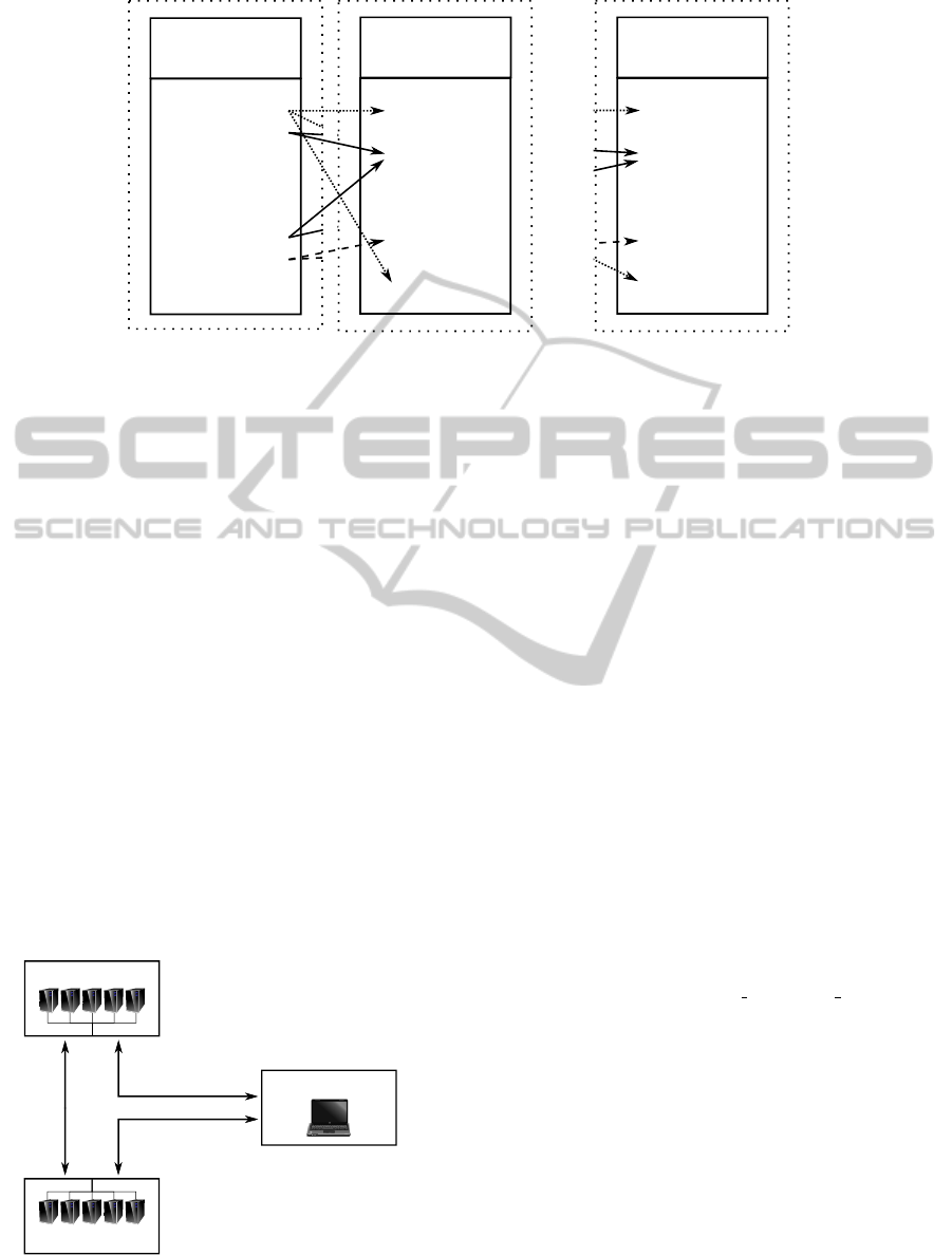
5 REMOTE SIMULATION

When the focus is on large-scale problems, it is not

uncommon that an optimization or simulation soft-

ware is tuned for a particular high-performance com-

puting system. In general, not all the optimization and

simulation software packages are available on all sys-

tems. We therefore suggest an approach based on dis-

tributed computing. This enables the combined use of

Simulation

Optimization

Steering/Setup

Figure 12: Remote object principle illustrating the general

possibilities for distributed computing in EFCOSS. (Clip-

arts from openclipart.org.)

(i) a dedicated simulation workstation or cluster, (ii)

a dedicated optimization workstation or cluster, and

(iii) a dedicated steering workstation. The resulting

remote object principle is shown in Fig. 12.

In this paper we focus on parallelism involved in

the simulation. We could also envision a situation

where the optimization algorithm is executed in par-

allel. However, the overall runtime is typically domi-

nated by the simulation and its derivatives rather than

by the optimization algorithm. So, we do not discuss

in this paper a distributed approach for a parallel op-

timization algorithm. Rather we consider distributed

computing for a parallel simulation. To this end, let

the optimization algorithm as well as the steering and

setup be serially executed on some machine. The sim-

ulation is then run on a different server, using an MPI-

parallelized code as discussed in the previous section.

We use the version 4.24 of the Python Remote

Object (PyRO) library (de Jong, 2013) for distribut-

ing Python objects. An example starting a simulation

server is shown in Fig. 13. This example shows the

MPI server code that starts a PyRO daemon on the

master process (rank=0). The other processes just

initialize the OptimizeSim class as stated before and

start the runtime loop with run function worker(),

shown in Fig. 9. As of PyRO version 4.18, the de-

fault serializer for sending objects is set to serpent.

This serializer is currently not capable of transferring

numpy data types. To overcome this issue, we con-

tinue to use the pickle serializer instead. Pickling is

a standard serialization protocol in Python, which has

drawbacks with respect to security. We assume that

this issue is solved in the next versions of PyRO so

that the serpent serializer can also transfer numpy

data types.

To correctly communicate with the remote simu-

lation server, the EFCOSS instance running the opti-

mization algorithm needs a new initialization method

ICSOFT-EA2014-9thInternationalConferenceonSoftwareEngineeringandApplications

452

from si m u lat i o n import Si m u l ati o n M P I

from Op t i miz e S i m import Op t i miz e S i m

import P yro 4

from m p i4p y import MPI

Py ro4 . c onf i g . SER I A L IZE R = ’ p i ck l e ’

Py ro4 . c onf i g . S E RIAL I Z E R S _ A C C EPTE D . a dd (

’ p ic k le ’)

def m ai n () :

co mm = MP I . COM M _ W ORL D

ra nk = com m . Ge t _ ran k ()

si ze = com m . Ge t _ siz e ()

if ( r an k == 0) :

si m u l ati o n = S i m u lat i o n M P I ( mod n ame =" sim ")

Py ro4 . D aem o n . ser v e S i mpl e (

{ simu l a tio n :

" e f cos s . S i mul a t ion " } ,

ns = Fa ls e )

else:

d= Opti m i z eSi m ()

d. init E F C OS S ()

d. ini t Sim ()

d. ru n _fun c t i o n _ w o rker ()

if _ _ n ame _ _ == " __ m ain _ _ ":

ma in ()

Figure 13: Python code for a remote MPI simulation server

using PyRO.

for the simulation. A corresponding code is given in

Fig. 14. This is a simple example illustrating the cre-

ation of a server process. Here, PyRO is used without

a nameserver. The PyRO object of the simulation is

retrieved by entering its universal resource identiﬁer

(URI), which the daemon prints on the remote ma-

chine.

def in i t S imRe m o t e ( se lf ) :

uri = inpu t (" Ent e r UR I of S i mul a t i on S erv e r : " ) .

st rip ()

sim = Pyro 4 . Pr o xy ( ur i )

sim . se t R e sul t V e c ( se lf . opt . g e tRe s u l t Vec () )

sim . se t Jac V e c ( se lf . opt . get J a cVe c () )

se lf . op t . s etSi m u l a t i o n Serv e r ( s im )

Figure 14: Python code to retrieve a remote object from the

simulation server.

6 CONCLUSIONS

An important class of problems arising in science

and engineering is to solve mathematical optimiza-

tion problems including data ﬁtting problems, where

a suitably-deﬁned objective function is minimized. A

typical objective function involves the evaluation of a

mathematical function that is represented by a com-

plicated simulation code. The scenario we consider

in this paper consists of bringing together an opti-

mization software package with a simulation package

via the simple and user-friendly software framework

EFCOSS, the Environment for Combining Optimiza-

tion and Simulation Software.

Today, many scientiﬁc and engineering software

packages involve some sort of parallelism. The

most prominent parallel programming paradigms are

OpenMP for shared-memory computers and MPI for

systems with distributed memory. With the help of

an illustrative example, we presented the feasibil-

ity of using EFCOSS to solve optimization problems

that involve simulation codes using either OpenMP or

MPI. Though not explicitly described, there is room

for another viable approach in which a combination

of OpenMP and MPI is used in a hybrid fashion. Fur-

thermore, EFCOSS facilitates distributed computing

by means of the publicly available Python Remote

Object package PyRO.

Similar to the coupling of a simulation software

package to EFCOSS, it is also relevant to consider

the situation where developers of optimization pack-

ages are interested in interfacing their software with

a simulation using EFCOSS. This is an ongoing work

which will be described elsewhere.

ACKNOWLEDGEMENTS

This work is partially supported by the German Fed-

eral Ministry for the Environment, Nature Conserva-

tion and Nuclear Safety (BMU) within the project

MeProRisk II, contract number 0325389 (F) as well

as by the German Federal Ministry of Education and

Research (BMBF) within the project HYDRODAM,

contract number 01DS13018.

REFERENCES

Averick, B. M., Carter, R. G., Mor

e, J. J., and Xue, G.-

L. (June 1992). The MINPACK-2 test problem col-

lection. Technical Report MCS–P153–0692, Argonne

National Laboratory.

Benson, S. J., Curfman McInnes, L., and Mor

e, J. J. (2001).

A case study in the performance and scalability of op-

timization algorithms. ACM Transactions on Mathe-

matical Software, 27(3):361–376.

Chapman, B., Jost, G., Van der Pas, R., and Kuck, D. J.

(2008). Using OpenMP: Portable shared memory

parallel programming. MIT Press, Cambridge, Mass.,

London.

Dalc

ın, L., Paz, R., and Storti, M. (2005). MPI for

Python. Journal of Parallel and Distributed Comput-

ing, 65(9):1108–1115.

de Jong, I. (2013). Pyro – Python Remote Objects.

http://pythonhosted.org/Pyro4.

Dennis, Jr., J. E. and Schnabel, R. B. (1983). Numerical

Methods for Unconstrained Optimization and Nonlin-

ear Equations. Prentice-Hall, Englewood Cliffs.

Fletcher, R. (1987). Practical Methods of Optimization.

John Wiley & Sons, New York, 2nd edition.

OntheDesignoftheEFCOSSSoftwareArchitectureWhenUsingParallelandDistributedComputing

453

Gay, D. M. (1990). Usage summary for selected optimiza-

tion routines. Computing Science Technical Report

153, AT&T Bell Laboratories.

Gill, P. E., Murray, W., and Wright, M. H. (1981). Practical

Optimization. Academic Press, New York.

Griewank, A. and Walther, A. (2008). Evaluating Deriva-

tives: Principles and Techniques of Algorithmic Dif-

ferentiation. Number 105 in Other Titles in Applied

Mathematics. SIAM, Philadelphia, PA, 2nd edition.

Gropp, W., Huss-Lederman, S., Lumsdaine, A., Lusk, E. L.,

Nitzberg, B., Saphir, W., and Snir, M. (1998). MPI–

The Complete Reference: Volume 2, The MPI-2 Ex-

tensions. MIT Press, Cambridge, MA, USA.

Hasco

et, L. and Pascual, V. (2013). The Tapenade au-

tomatic differentiation tool: Principles, model, and

speciﬁcation. ACM Trans. Math. Softw., 39(3):20:1–

20:43.

Henning, M. (2008). The rise and fall of CORBA. Commu-

nications of the ACM, 51(8):52–57.

Kenny, J. P., Benson, S. J., Alexeev, Y., Sarich, J.,

Janssen, C. L., Curfman McInnes, L., Krishnan, M.,

Nieplocha, J., Jurrus, E., Fahlstrom, C., and Windus,

T. L. (2004). Component-based integration of chem-

istry and optimization software. Journal of Computa-

tional Chemistry, 25(14):1717–1725.

orkel, S. (2002). Numerische Methoden f

ur Optimale

Versuchsplanungsprobleme bei nichtlinearen DAE-

Modellen. PhD thesis, University of Heidelberg, Ger-

many.

Lawrence, C. T. and Tits, A. L. (1996). Nonlinear equality

constraints in feasible sequential quadratic program-

ming. Optimization Methods and Software, 6:265–

282.

Lindstr

om, P. and Wedin, P.-

A. (1999). Gauss-Newton

based algorithms for constrained nonlinear least

squares problems. Department of Computing Science,

Faculty of Science and Technology, Ume

a University,

Sweden.

Munson, T., Sarich, J., Wild, S., Benson, S., and Curfman

McInnes, L. (2012). TAO 2.0 users manual. Technical

Report ANL/MCS–TM–322, Mathematics and Com-

puter Science Division, Argonne National Laboratory.

http://www.mcs.anl.gov/tao.

Nocedal, J. and Wright, S. J. (2006). Numerical Optimiza-

tion. Springer, New York, 2nd edition.

Object Management Group (2012). Common Object Re-

quest Broker Architecture (CORBA): Speciﬁcation,

Version 3.3. http://www.omg.org/spec/CORBA/3.3.

Oliphant, T. E. (2007). Python for scientiﬁc computing.

Computing in Science & Engineering, 9(3):10–20.

OpenMP Architecture Review Board (2013). OpenMP

Application Program Interface, Version 4.0.

http://www.openmp.org.

Pukelsheim, F. (2006). Optimal Design of Experiments.

Number 50 in Classics in Applied Mathematics.

SIAM, Philadelphia.

Rall, L. B. (1981). Automatic Differentiation: Techniques

and Applications, volume 120. Springer Verlag,

Berlin.

Rasch, A. and B

ucker, H. M. (2010). EFCOSS: An interac-

tive environment facilitating optimal experimental de-

sign. ACM Transactions on Mathematical Software,

37(2):13:1–13:37.

Seidler, R., B

ucker, H. M., Padalkina, K., Herty, M.,

Niederau, J., Marquart, G., and Rasch, A. (2014).

Redesigning the EFCOSS framework towards ﬁnding

optimally located boreholes in geothermal engineer-

ing. In Horv

at, I. and Rus

ak, Z., editors, Proceed-

ings of the tenth international symposium on tools and

methods of competetive engineering (TMCE 2014),

May 19–23, 2014, Budapest, Hungary, pages 831–

842.

Snir, M., Otto, S., Huss-Lederman, S., Walker, D., and Don-

garra, J. (1995). MPI–The Complete Reference. MIT

Press, Cambridge, MA, USA.

Snir, M., Otto, S. W., Huss-Lederman, S., Walker, D. W.,

and Dongarra, J. (1998). MPI–The Complete Refer-

ence: Volume 1, The MPI Core. MIT Press, Cam-

bridge, MA, USA, 2nd edition.

The Scipy Community (2013). SciPy v0.13.0 reference

guide.

Wedin, P.-

A. and Lindstr

om, P. (1988). Methods and soft-

ware for nonlinear least squares problems. Technical

Report UMINF–133.87, Inst. of Information Process-

ing, University of Ume

a, Ume

a, Sweden.

ICSOFT-EA2014-9thInternationalConferenceonSoftwareEngineeringandApplications

454