
Fluid Mechanics for Path Planning and Obstacle Avoidance
of Mobile Robots
Rainer Palm and Dimiter Driankov
AASS,
¨
Orebro University, SE-70182,
¨
Orebro, Sweden
Keywords:
Mobile Robots, Obstacle Avoidance, Fluid Mechanics, Velocity Potential.
Abstract:
Obstacle avoidance is an important issue for off-line path planning and on-line reaction to unforeseen ap-
pearance of obstacles during motion of a non-holonomic mobile robot along a predefined trajectory. Possible
trajectories for obstacle avoidance are modeled by the velocity potential using a uniform flow plus a doublet
representing a cylindrical obstacle. In the case of an appearance of an obstacle in the sensor cone of the robot a
set of streamlines is computed from which a streamline is selected that guarantees a smooth transition from/to
the planned trajectory. To avoid collisions with other robots a combination of velocity potential and force
potential and/or the change of streamlines during operation (lane hopping) are discussed.
1 INTRODUCTION
Obstacle avoidance is important for off-line plan-
ning and on-line reaction to unforeseen and sud-
den appearance of obstacles during motion of non-
holonomic mobile robots. Several methods have
been applied to obstacle avoidance in the artificial
force potential field method introduced by Khatib in
1985 (Khatib, 1985). The idea is to introduce arti-
ficial attractive and repulsive forces that enable the
robot to move around an obstacle while aiming at
a final target at the same time. Optimization tech-
niques like market-based optimization (MBO) parti-
cle swarm optimization (PSO) influencing artificial
potential fields have been presented by Palm and
Bouguerra (R.Palm and Bouguerra, 2011; Palm and
Bouguerra, 2013a). Other approaches have been pre-
sented by Borenstein (Borenstein and Koren, 1991),
who introduced the vector field histogram technique,
and Michels (Michels et al., 2005) who applied the re-
inforcement learning method. Specific ad hoc heuris-
tics have been proposed by Fayen (B.R.Fayen and
W.H.Warren, 2003) and Becker (Becker et al., 2006).
Despite of the simplicity and elegance of the ar-
tificial force potential field method the risk of dead-
locks (local minima) or undesired movements in the
vicinity of obstacles should be realized. Reinforce-
ment learning may be able to cope with this drawback
but to the costs of a high computational effort.
Another kind of artificial potential for obsta-
cle avoidance was therefore introduced by Khosla
(Khosla and Volpe, 1988) who used the velocity po-
tential of fluid mechanics to construct stream lines
in a working area of a mobile robot moving around
obstacles in a very natural way. The velocity poten-
tial approach is a method which considers both the
path/trajectory planning in the case of a well known
scenario including static obstacles and the on-line re-
action to unplanned situations like obstacle avoidance
in an unknown terrain.
Kim and Khosla continued this work with the use
of the velocity potential function to avoid obstacles
in real time (Kim and Khosla, 1992). Further sim-
ilar research has been published by Li et al (Li and
Bui, 1998), Ge et al (Ge and Cui, 2002), Waydo
and Murray (Waydo and Murray, 2003), Daily and
Bevly (Daily and Bevly, 2008), Sugiyama (Sugiyama
and Akishita, 1998), (Sugiyama et al., 2010), Gin-
gras et al (Gingras et al., 2010), and Owen et al
(Owen et al., 2011). Most of these approaches use
a point source/point sink combination for flow con-
struction. This can be of disadvantage in the presence
of a combination of tracking velocity vectors and ob-
stacle avoidance vectors.
Therefore in this paper the uniform flow of a fluid
around an obstacle is preferred. Possible trajectories
for obstacle avoidance are modeled by the velocity
potential using a uniform flow plus a doublet repre-
senting a cylindrical obstacle. The motion of a non-
holonomic mobile robot is firstly defined by a pre-
defined trajectory. In the case of an appearance of
one or more obstacles in the sensor cone of the robot
231
Palm R. and Driankov D..
Fluid Mechanics for Path Planning and Obstacle Avoidance of Mobile Robots.
DOI: 10.5220/0004986902310238
In Proceedings of the 11th International Conference on Informatics in Control, Automation and Robotics (ICINCO-2014), pages 231-238
ISBN: 978-989-758-040-6
Copyright
c
2014 SCITEPRESS (Science and Technology Publications, Lda.)
a set of streamlines is computed from which those
streamline is selected that guarantees a smooth transi-
tion from the planned trajectory to the streamline and,
after having left behind the obstacle, back to the orig-
inal trajectory. To avoid collisions with other moving
obstacles (e.g. robots) a combination of velocity po-
tential and force potential is discussed. In the case of
possible collisions between robots moving on cross-
ing streamlines a change between streamlines during
operation (lane hopping) is presented.
2 MODELING OF THE SYSTEM
2.1 Kinematics
We consider a non-holonomic rear-wheel driven vehi-
cle with the kinematics of a car. The kinematic of the
non-holonomic vehicle is described by
˙q
i
= R
i
(q
i
) · u
i
q
i
= (x
i
, y
i
, Θ
i
, ϕ
i
)
T
(1)
R
i
(q
i
) =
cosΘ
i
0
sinΘ
i
0
1
l
i
· tanϕ
i
0
0 1
where
q
i
∈ ℜ
4
- state vector
u
i
= (u
1
i
, u
2
i
)
T
∈ ℜ
2
- control vector, push-
ing/steering speed
x
i
p
= (x
i
, y
i
)
T
∈ ℜ
2
- position vector of platform P
i
Θ
i
- orientation angle
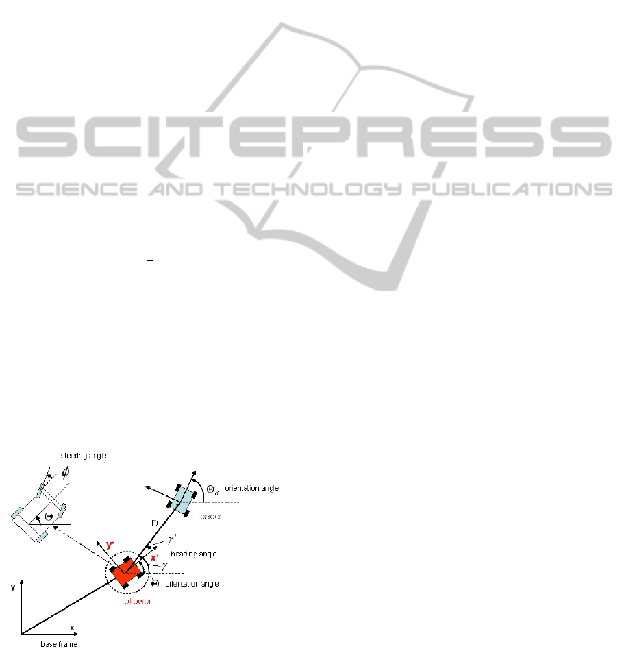
ϕ
i
- steering angle
l
i
- length of vehicle
Figure 1: Leader follower principle.
2.2 Virtual Leader
Many tracking methods use a predefined path or a
trajectory as a control reference for the vehicle to be
controlled. In contrast to this a ’virtual’ vehicle (the
leader) is introduced that moves in front of the ’real’
vehicle (the follower) (see also (Leonard and Fiorelli,
2001)). The virtual leader acts as trajectory generator
for the real platform at every time step, based on start-
ing and end position (target), obstacles to be avoided,
other platforms to be taken into account etc (see Fig.
1). The dynamics of the virtual platform is designed
as a first order system that automatically avoids abrupt
changes in position and orientation
˙v
vi
= k
vi
(v
vi
− v
di
) (2)
v
vi
∈ ℜ
2
- velocity of virtual platform P
i
v
di
∈ ℜ
2
- desired velocity of virtual platform P
i
k
vi
∈ ℜ
2×2
- damping matrix (diagonal)
v
di
is composed of the tracking velocity v
ti
and
velocity terms due to artificial potential fields from
obstacles and other platforms The tracking velocity is
designed as a control term
v
ti
= k
ti
(p
x
i
− x
ti
) (3)
x
ti
∈ ℜ
2
- position vector of target T
i
p
x
i
∈ ℜ
2
- position vector of platform P
i
k
ti
∈ ℜ
2×2
- gain matrix (diagonal)
There are many ways of computing the control
vector u
i
for the follower in (1). Under the assump-
tion of a slowly time varying ’leader-follower’ system
a local linear gain scheduler is applied that is designed
according to (Palm and Bouguerra, 2013b).
3 SOME PRINCIPLES OF FLUID
MECHANICS
A closer look at the problem of path planning and
obstacle avoidance leads to a similar case when flu-
ids circumvent obstacles in a smooth and energy sav-
ing way. The result is a bundle of trajectories from
which one can conclude how an autonomous robot
should behave under non-holonomic constraints. In
the theory of fluids the terms velocity potential,
stream function and complex potential are introduced
(Nakayama, 1999). The so-called uniform parallel
flow is introduced that corresponds to an undisturbed
trajectory along straight lines. The flow of a doublet
corresponds to a flow around a cylinder. Superposi-
tion of uniform flow and doublet leads to a model of a
uniform flow around a cylindrical obstacle.
ICINCO2014-11thInternationalConferenceonInformaticsinControl,AutomationandRobotics
232
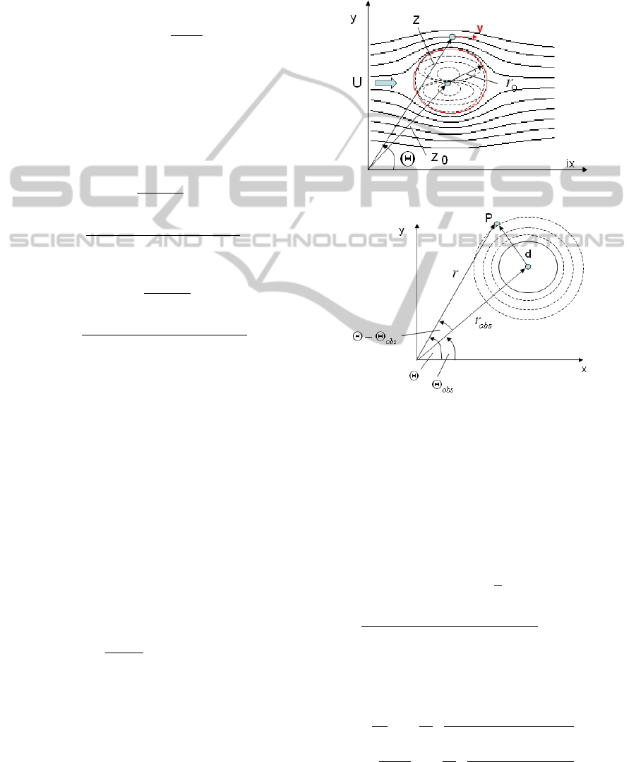
3.1 Superposition of Uniform Flow and
Doublet
The flow around a cylindrical object - an obstacle -
is finally computed by a superposition of the uniform
flow and the doublet which is a superposition of their
complex potentials (see Fig. 2).
w(z) = U · z +U
r
2
0
z − z
0
(4)
where U is the flow, r
0
is the radius of the obstacle
z = r(cosΘ + isinΘ) is the complex variable. z
0
is the
position of the obstacle in the complex plane, Θ is
the angle between z and the imaginary axis (see Fig.
2 ) The velocity components in polar coordinates are
obtained as
v
r
= U · ((1 +
r
2
0
z
2
re
+ z
2
im
)cosΘ (5)
−
2z
re
· r
2
0
(z
re
cosΘ + z
im
sinΘ)
(z
2
re
+ z
2
im
)
2
)
v
Θ
= −U · ((1 +
r
2
0
z
2
re
+ z
2
im
)sinΘ (6)
+
2z
re
· r
2
0
(−z
re
sinΘ + z
im
cosΘ)
(z
2
re
+ z
2
im
)
2
)
where z
re
= rcosΘ−x
0
and z
im
= rsin Θ −y
0
. Here
one has to mention that stream lines not only exist
outside but also inside the cylinder. The speciality
of this flow model is that the surface of the cylinder
itself is a streamline. Therefore one can ignore the
stream lines inside the cylinder because the surface
of the cylinder serves as a borderline for stream lines
that cannot be trespassed.
3.2 Superposition of Two or More
Cylinders
For more than one cylinder weighting functions µ
i
for
the flows U
i
are introduced depending on the distance
of the actual robot position d
i
to the cylinder surfaces
(Waydo and Murray, 2003), (Daily and Bevly, 2008)
µ
i
=
∏
i̸= j
d
j
d
i
+ d
j
; U
i
= µ
i
·U (7)
From (5), (6), and (7) one obtains velocity compo-
nents v
r
i
and v
Θ
i
in polar coordinates that will be
transformed into cartesian coordinates by
(u
i
, v
i
)
T
=
(
cos(Θ) −sin(Θ)
sin(Θ) cos(Θ)
)
· (v
r
i
, v
Θ
i
)
T
(8)
Summerizing the velocities u
i
in x-direction and
v
i
in y-direction in cartesian coordinates
u
tot
=
∑
i
u
i
v
tot
=
∑
i
v
i
(9)
leads to the streamlines for the multiple obstacle case.
Figure 2: Flow around a cylinder.
Figure 3: Force potential.
3.3 Comparison between Velocity and
Force Potential
In the following a comparison between velocity and
force potential shows the contrasts and the similari-
ties between these two types of potentials. The force
potential of a circular object (see Fig. 3) is given by
p
f orce
=
c
d
(10)
with c - strength of potential field
d =
√
r
2
− 2rr
obs
cos(Θ − Θ
obs
) + r
2
obs
For a point P(r, Θ) the repulsive force and - with
this - the repulsive velocity v
rep
= (v
r
, v
Θ
)
T
yields
v
r
=
d p
dr
= −
c
d
2
·
r − r
obs
· cos(Θ − Θ
obs
)
d
(11)
v
Θ
=
d p
r · dΘ
= −
c
d
2
·
r
obs
· sin(Θ − Θ
obs
)
d
(12)
FluidMechanicsforPathPlanningandObstacleAvoidanceofMobileRobots
233
Compared with the flow of a doublet and the corre-
sponding velocities (5) and (6) we can conclude that
these two concepts are different but also have com-
mon features: after some conversions the force po-
tential appears as a term in the velocity potential. A
crucial point, however, is that for the force potential
the ”streamlines” always point in the direction away
from the ”gravity center”. By contrast for the veloc-
ity potential field the stream lines Ψ always have a
tangential component This is of great advantage for
obstacle avoidance because it helps a mobile vehi-
cle to move around the obstacle in an optimal way
in the sense that the streamlines are symmetrical with
respect to the axis perpendicular to the flow going
through the ”poles” of the cylinder. However a com-
bination of velocity and force potential should also be
considered. Such a combination takes place if dur-
ing tracking along a streamline an unforeseen moving
obstacle - e.g. another robot - appears in the sensor
cone. In this case the current trajectory given by the
actual streamline is corrected by the repulsive force of
the moving obstacle.
4 OBSTACLE AVOIDANCE USING
THE VELOCITY POTENTIAL
The previous calculations of the velocity potential are
performed in a coordinate frame corresponding to the
local robot frame. In the multi-robot case this con-
cerns every involved robot so that a total view of the
whole scenario can only be obtained from the view-
point of the base frame.
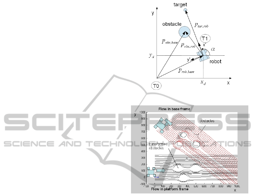
Figure 4 shows the relationship between the robot
frame T1 and the base frame T0. The transformation
matrix between T1 and T0 is
A
10
=
cos(α) −sin(α) x
d
sin(α) cos(α) y
d
0 0 1
(13)
To compute the streamline array v
f low,rob
=
(v
r
, v
Θ
, 1)
T
in the base frame the following steps are
necessary:
1. Transform the obstacle coordinates into the robot
frame
p
obs,rob
= A
−1
10
· p
obs,base
(14)
2. Calculate the streamline arrays v
f low,rob
(k), k -
discrete time step, from eqs. (5) and (6) in T1
and the corresponding flow trajectory p
f low,rob
(k)
of the flow.
Figure 4: Relations between frames.
Figure 5: Transformation between frames.
3. Transform the flow trajectory p
f low,rob
into the
base frame T0
p
f low,base
(k) = A
10
· p
f low,rob
(k) (15)
Figure 5 shows the particular stages of the computa-
tion of stream lines.
Remark: A stagnation point near the obstacle
should be recognized in a very early stage. A cor-
responding test is relatively simple and is to be done
in the robot frame for every streamline: Check the
x-coordinate x
end
i
of the endpoint of streamline i rela-
tive to the x-coordinate x
obs
of the obstacle. If x
end
i
≤
x
obs
then the regarding streamline ends up with a stag-
nation point and should be excluded. A more conser-
vative test is x
end
i
≤ x
obs
+ C, where C is a positive
number, e.g. C = 2 · r
0
After that, those streamline is selected for the
robot which lies closest to the original predefined
trajectory. In order to get a smooth connection to
the original trajectory the following transition filter is
used
ICINCO2014-11thInternationalConferenceonInformaticsinControl,AutomationandRobotics
234
p
x
(k + 1) = p
x
(k) + K
f ilt
· (x
array
(k + 1) − p
x
(k))
(16)
where p
x
(k) ∈ ℜ
2
- actual position of robot,
x
array
(k) = p
f low,base
(k), K
f ilt
∈ ℜ
2×2
- filter matrix.
For the change from a streamline to the original tra-
jectory we have to consider two cases:
1. A trajectory x
tra j
(k) is defined between starting
point x
tra j
(1) and endpoint x
tra j
(k
end
).
2. Only the target endpoint x
tra j
plus constraints upon
the velocities v = (u, v)
T
are defined.
Case 1 is difficult to solve because the original tra-
jectory is cut into 3 parts: a part before entering the
streamlines with k = 1...k
in
, a part which is covered
by the area of streamlines with k = k
in
...k
tr,out
, and
a part with k = k
tr,out
...k
end
after the area of stream-
lines. Suppose that the trajectory leaves the area
of streamlines between two endpoints of streamlines.
x
tra j
(k
in
) be the point on the trajectory at k
in
when the
robot (and the trajectory) enters the area of stream-
lines. x
tra j
(k
tr,out
) is the point on the trajectory at
k
tr,out
when the trajectory leaves the area of stream-
lines. x
tra j
(k
end
) is the end of the trajectory at k
end
.
At first one has to search for the first trajectory point
x
tra j
(k
tr,out
) after having left the area of streamlines
(see Fig. 6). A solution to this is the following:
1. Transform the total trajectory x
tra j
(k) into the robot
frame T1
x
tra j
rob
(k) = A
01
(k
out
) · x
tra j
(k) (17)
A
01
= A
−1
10
; k = 1...k
end
where k
out
is the time point for the robot to leave the
area of streamlines.
2. Search for the first trajectory point for which
x
tra j
rob
(k) > 0; k > k
in
. The result is x
tra j
rob
(k
tr,out
).
Choose another trajectory point x
tra j
rob
(k
tr,out
1
) >
x
tra j
rob
(k
tr,out
); k
tr,out
1
> k
tr,out
to enable a smoother
transition.
3. Activate a transition filter
p
x
(k + 1) = (18)
p
x
(k) + K
f ilt
· (x
tra j
(k
tr,out
1
+ k) − p
x
(k))
where k = 1...(k
end
− k
tr,out
1
), which guarantees a
smooth transition to the original trajectory.
Case 2 is simpler: once having left a streamline
it is immediately possible for the robot to move to
the target x
tra j
. We introduce another transition fil-
ter which guarantees a smooth transition between a
streamline and the target. Let p
x
(k
out
) be the position
of the robot at the end of the streamline. Then we
obtain for the transition filter
p
x
(k + 1) = p
x
(k) + K
f ilt
· (x
tra j
(k
end
) − p
x
(k)) (19)
where k ≥ k
out
.
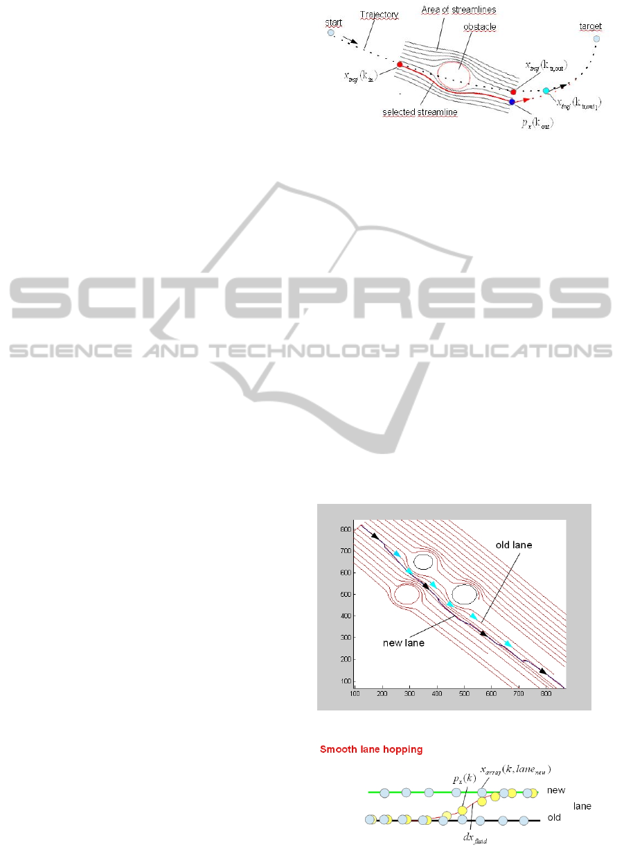
Figure 6: Transition between trajectory and streamline.
5 CHANGING STREAMLINES
DURING OPERATION (LANE
HOPPING)
First of all it has to be stressed that the change of a
streamline during operation (lane hopping) becomes
feasible if several streamlines are computed in ad-
vance. Each streamline constitutes a possible trajec-
tory for the mobile platform. Once a streamline is se-
lected for a platform it may be necessary to leave the
actual streamline (lane) during operation and change
to another one because of the following reasons:
1. The platform is too close to a static obstacle
2. The streamline violates hard/soft constraints
3. The platform is expected to collide with another
moving obstacle (platform)
Figure 7: Change of streamline (lane hopping).
Figure 8: Principle of lane hopping.
FluidMechanicsforPathPlanningandObstacleAvoidanceofMobileRobots
235
Lane hopping means the change from the cur-
rent streamline to another streamline which may be
a neighboring streamline but not necessarily. Figure
7 presents a case where the robot changes the stream-
lines to avoid a motion too close to the obstacles. This
change should not be too abrupt but rather a smooth
transition (see Fig. 8). This is again realized by a filter
function either in the robot or world frame
dx
f luid
(k + 1) =
K
f ilt
· (x
array
(k + 1|lane
new
) − p
x
(k)) (20)
p
x
(k + 1) = p
x
(k) + dx
f luid
(k + 1)
where it is assumed that the x-positions in the
robot frame x
array
(k|lane
old
) ≈ x
array
(k|lane
new
). If
x
array
(k|lane
old
) > x
array
(k|lane
new
) then (20) has to
be corrected to
dx
f luid
(k + 1) = K
f ilt
· (x
array
(k + δ|lane
new
) − p
x
(k))
(21)
δ is the number of time steps for which
x
array
(k|lane
old
) ≈ x
array
(k + δ|lane
new
) (22)
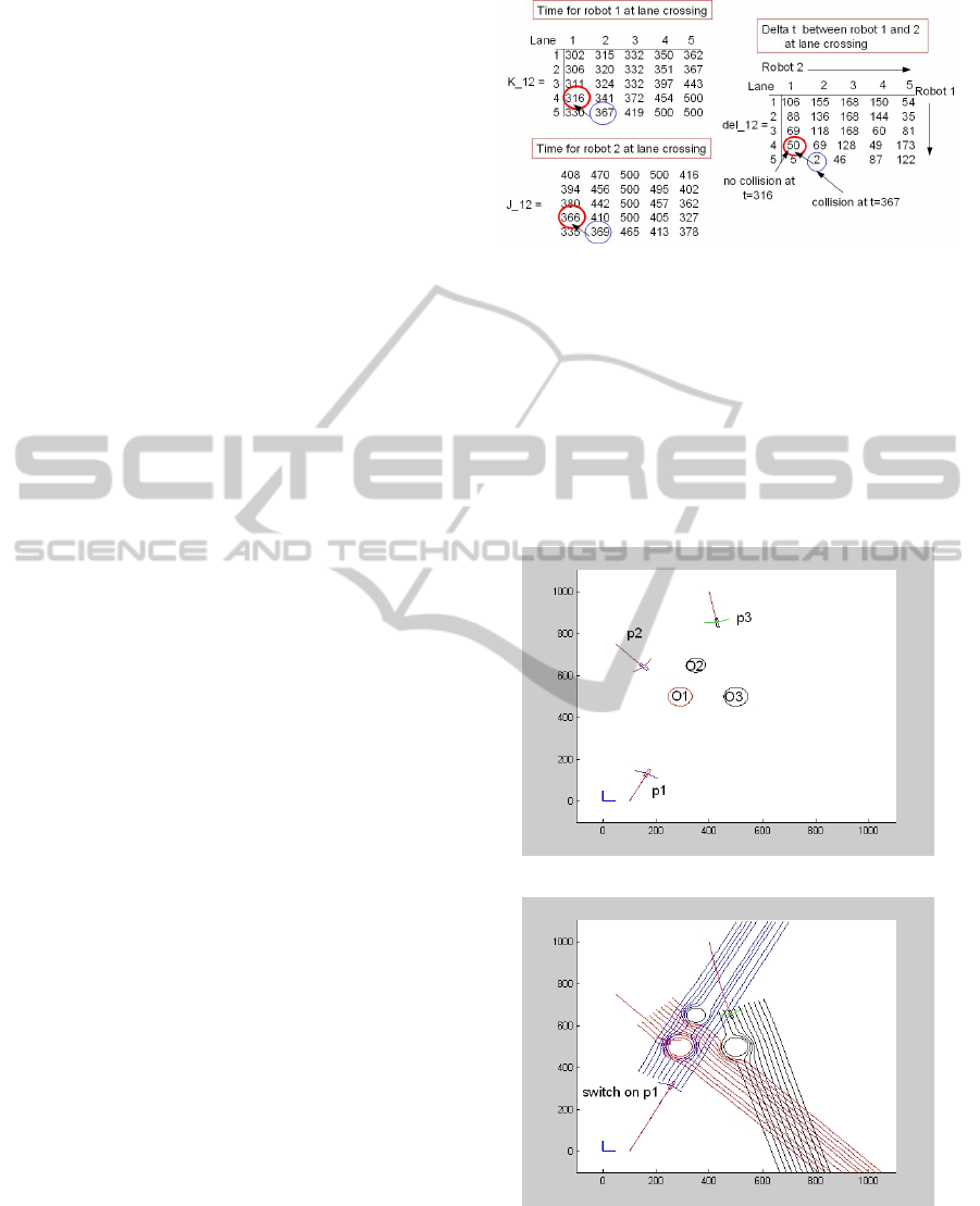
In the case of a global (centralized) control of the
robot fleet it is possible to compute possible collisions
of platforms in advance if they would keep on moving
on the originally chosen lanes. Let us compare the 5
lanes each of platforms 1 and 2 and calculate the dis-
crete time stamps at their crossings, and the difference
between these time stamps. Let for example robot 1
move on lane 5 and robot 2 on lane 2. Lanes 5 and 2
cross at t = 367 for robot 1 (see Fig. 9, matrix K12,
blue circle) and for robot 2 at t = 369 (see matrix J12,
blue circle) . The distance between the two entries is
2 (see Fig. 9, matrix del12) which points to a collision
at time t ≈ 367.
In order to avoid a collision many different options
are possible. We have chosen the following option:
robot 1 → lane 4, robot 2 → lane 1. The result can
also be observed in Fig. 9, red circles. The difference
(distance) between the time stamps t = 316 for robot
1 and t = 366 for robot 2 is 50 which is sufficient for
avoiding a collision. See also Figs. 14 and 15
6 SIMULATION RESULTS
The simulation shows 3 mobile robots (platforms)
aiming at their targets (see Fig. 10), crossing ar-
eas of 3 obstacles while sharing a common working
area for some time. Platform p2 switches on first its
streamline because obstacle O1 is first detected. Then
follows p3 seeing O3 in its sensor cone and finally
p1 with O1 in its sensor cone (see Fig. 11). Then
Figure 9: Simulation example, with/without lane hopping.
the platforms ’switch off’ their streamlines in the se-
quence p1, p3, p2 (because the obstacles disappear
from their sensor cones) and reach finally their targets
(see Fig. 12). The final trajectories show the inter-
play of different influences from planned trajectories,
streamlines, and artificial force fields in the case when
robots avoid each other. Figure 13 shows the regard-
ing velocity profiles of the individual robots and the
switching sequence of the streamlines.
Figure 10: No stream lines on.
Figure 11: All platforms streamlines on.
As to the change of streamlines (lane hopping) the
imminent danger of a collision between robots 1 and
2 is shown in Fig. 15. Figure 15 shows that lane hop-
ping avoids a collision between robots 1 and 2 pro-
ICINCO2014-11thInternationalConferenceonInformaticsinControl,AutomationandRobotics
236
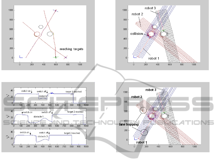
Figure 12: Platforms reach targets.
Figure 13: Velocity profiles.
vided that the change of the lanes takes place in a suf-
ficient distance to the possible collision. A practical
solution is the following:
- Check the time t
cross
to a possible collision
- Calculate the time t
change
to change between two
neighboring lanes
- Start changing at least 2 · t
change
before possible
crossing
If it is not sufficient to change to a neighboring lane
then apply the same procedure to another lane while
taking into account longer changing times because of
the longer distance between the lanes.
7 CONCLUSIONS
Fluid mechanics and its velocity potential principle is
a powerful mean both for path planning and sensor
guided on-line reaction to obstacles. The velocity po-
tential has been used for avoiding static obstacles to-
gether with the force potential for moving obstacles.
Finally it has been shown that the change of stream-
lines during operation can avoid imminent collisions
Figure 14: Simulation example, no lane hopping.
Figure 15: Simulation example, with lane hopping.
between robots. This change is done in a smooth
way and at an early stage before a possible collision.
To avoid possible collisions between robots moving
on crossing streamlines a change between streamlines
during operation (lane hopping) is presented. A crit-
ical aspect is that obstacles are very rarely cylindri-
cal. This, however, can easily be handled by a rough
approximation of the obstacle by an appropriate num-
ber of cylinders. The driveable streamlines are then
lying at the edges (left or right) of the conglomerate
of cylinders (Daily and Bevly, 2008). The computa-
tional effort of the method is mainly determined by
equations (5, 6, 8, 14, 15) computed for n streamlines
and m time steps but only at the moment of the detec-
tion of an obstacle. A future work lies therefore in the
modeling of the stream lines to make the use of the
approach easier for real applications.
REFERENCES
Becker, M., Dantas, C., and Macedo, W. (2006). Obsta-
cle avoidance procedure for mobile robots. In ABCM
Symposium in Mechatronics, vol. 2. ABCM.
Borenstein, J. and Koren, Y. (June 1991). The vector field
FluidMechanicsforPathPlanningandObstacleAvoidanceofMobileRobots
237

histogram - fast obstacle avoidance for mobile robots.
IEEE Trans. on Robotics and Automation, Vol. 7, No
3, pages 278–288.
B.R.Fayen and W.H.Warren (2003). A dynamical model
of visually-guided steering, obstacle avoidance, and
route selection. International Journal of Computer Vi-
sion, 54(1/2/3), page 1334.
Daily, R. and Bevly, D. M. (2008). Harmonic potential
field path planning for high speed vehicles. American
Control Conference, 2008, Seattle, Washington, USA,
pages 4609 – 4614.
Ge, S. and Cui, Y. (2002). Dynamic motion planning
for mobile robots using potential field method. Au-
tonomous Robots, 13, pages 207 – 222.
Gingras, D., Dupuis, E., Payre, G., and Lafontaine, J.
(2010). Path planning based on fluid mechanics for
mobile robots using unstructured terrain models. In
Proceedings ICRA 2010. ICRA 2010.
Khatib, O. (1985). Real-time 0bstacle avoidance for ma-
nipulators and mobile robots. IEEE Int. Conf. On
Robotics and Automation,St. Loius,Missouri, 1985,
page 500505.
Khosla, P. K. and Volpe, R. (1988). Superquadric avoidance
potentials for obstacle avoidance. In IEEE Conference
on Robotics and Automation, Philadelphia PA. IEEE,
Springer-Verlag London.
Kim, J.-O. and Khosla, P. K. (1992). Real-time obstacle
avoidance using harmonic potential functions. IEEE
Trans on Robotics and Automation,, pages 1–27.
Leonard, N. E. and Fiorelli, E. (Dec 2001). Virtual leaders,
artificial potentials and coordinated control of groups.
Proc. of the 40th IEEE Conf. on Decision and Control,
Orlanda, Florida USA, pages 2968–2973.
Li, Z. X. and Bui, T. D. (1998). Robot path planning using
fluid model. Journal of Intelligent and Robotic Sys-
tems, vol. 21, pages 29–50.
Michels, J., Saxena, A., and Ng, A. Y. (2005). High speed
obstacle avoidance using monocular vision and re-
inforcement learning. 22nd Int’l Conf on Machine
Learning (ICML), Bonn, Germany.
Nakayama, Y. (1999). Introduction to fluid mechanics.
Butterworth-Heinemann, Oxford Auckland Boston.
Owen, T., Hillier, R., and Lau, D. (2011). Smooth path plan-
ning around elliptical obstacles using potential flow
for non-holomonic robots. In Robocup 2011: Soccer
World Cup XV, volume 7416.
Palm, R. and Bouguerra, A. (2013a). Particle swarm opti-
mization of potential fields for obstacle avoidance. In
Proceeding of RARM 2013, Istanbul, Turkey. Volume:
Scient. coop. Intern. Conf. in elect. and electr. eng.
Palm, R. and Bouguerra, A. (2013b). Particle swarm opti-
mization of potential fields for obstacle avoidance. In
Proc. of RARM 2013, Istanbul 09/2013.
R.Palm and Bouguerra, A. (2011). Navigation of mobile
robots by potential field methods and market-based
optimization. ECMR 2011 , Oerebro, Sweden.
Sugiyama, S. and Akishita, S. (1998). Path planning for mo-
bile robot at a crossroads by using hydrodynamic po-
tential. In Proc. of 1998 JAPAN-U.S.A SYMPOSIUM
ON FLEXIBLE AUTOMATION.
Sugiyama, S., Yamada, J., and Yoshikawa, T. (2010). Path
planning of a mobile robot for avoiding moving ob-
stacles with improved velocity control by using the
hydrodynamic potential. IEEE/RSJ Intern. Conf. on
Intell. Robots and Systems, page 207222.
Waydo, S. and Murray, R. M. (2003). Vehicle motion plan-
ning using stream functions. In Proc. IEEE Int. Conf.
Rob. Autom., volume 2. IEEE.
ICINCO2014-11thInternationalConferenceonInformaticsinControl,AutomationandRobotics
238
