Signature-based High-level Simulation of Microthreaded Many-core

Architectures

Irfan Uddin, Raphael Poss and Chris Jesshope

Computer Systems Architecture group, Informatics Institute, University of Amsterdam,

Sciencepark 904, 1098 XH Amsterdam, The Netherlands.

Keywords:

Performance estimation, many-core systems, high-level simulations.

Abstract:

The simulation of ﬁne-grained latency tolerance based on the dynamic state of the system in high-level simu-

lation of many-core systems is a challenging simulation problem. We have introduced a high-level simulation

technique for microthreaded many-core systems based on the assumption that the throughput of the program

can always be one cycle per instruction as these systems have ﬁne-grained latency tolerance. However, this

assumption is not always true if there are insufﬁcient threads in the pipeline and hence long latency operations

are not tolerated. In this paper we introduce Signatures to classify low-level instructions in high-level cate-

gories and estimate the performance of basic blocks during the simulation based on the concurrent threads in

the pipeline. The simulation of ﬁne-grained latency tolerance improves accuracy in the high-level simulation

of many-core systems.

1 INTRODUCTION

Maintaining accuracy in the high-level simulation of

single-core systems is a difﬁcult simulation problem.

This problem becomes challenging in many-core sys-

tems, where the throughput of a program depends on

the dynamic state of the system. The problem is fur-

ther exacerbated in a multi-threaded many-core sys-

tems, where multiple threads may be able to hide the

latency of long latency operations reducing the num-

ber of cycles per instruction in the throughput of the

program. For example a ﬂoating point operation may

take cycles to complete when there is only one thread

in the pipeline, or these cycles may be decreased with

the increasing number of threads.

In this paper we present a high-level simulation

technique for the ﬁne-grained latency tolerance in mi-

crothreaded many-core systems. We identify different

low-level instructions of the architecture and classify

them into high-level classes referred as signatures.

This classiﬁcation is made based on the number of

cycles taken by different instructions and how the cy-

cles can be tolerated based on the number of threads

currently active per core. Signatures are then used

in the high-level simulator to adapt the throughput of

the program during simulation to more accurately es-

timate program’s workload.

The simulation technique can be used in the high-

level simulation of ﬁne-grained latency tolerance in

many-core systems. As long as we can track the num-

ber of active threads in the high-level simulation, the

signature of a basic block can be used to improve the

estimated simulated time of that basic block. Some of

the modern many-core systems with latency tolerance

are The Microgrid, TILE64, Sun/Oracle UltraSPARC

Tx series etc. In this paper, we present the simulation

technique to simulate the ﬁne-grained latency toler-

ance in the context of the microthreaded many-core

systems which uses a multi-threaded processor with

data-ﬂow synchronization and is able to tolerate la-

tencies of up to thousands of cycles in a typical con-

ﬁguration (Bousias et al., 2009).

The rest of the paper is organized as follows.

We give a background to the microthreaded architec-

ture, cycle-accurate simulation and high-level simu-

lation in section 2. We introduce signatures in sec-

tion 3, ﬁne-grained latency tolerance in the mi-

crothreaded architecture in section 4 and its simula-

tion in section 5. We present results collected from

the Signature-based high-level simulation framework

in section 6 and conclude the paper in section 7.

509

Uddin I., Poss R. and Jesshope C..

Signature-based High-level Simulation of Microthreaded Many-core Architectures.

DOI: 10.5220/0004982405090516

In Proceedings of the 4th International Conference on Simulation and Modeling Methodologies, Technologies and Applications (SIMULTECH-2014),

pages 509-516

ISBN: 978-989-758-038-3

 2014 SCITEPRESS (Science and Technology Publications, Lda.)

2 BACKGROUND

The Microgrid (Jesshope, 2004; Bernard et al., 2011;

Jesshope, 2008) is a general-purpose many-core ar-

chitecture and implements hardware multithreading

using data-ﬂow scheduling with a concurrency man-

agement protocol in hardware to create and synchro-

nize threads within and across cores on a chip. The

programming model for the architecture is called the

microthreading model. Each core of the Microgrid

contains a single issue, in-order RISC pipeline with

an ISA similar to DEC/Alpha, and all cores are con-

nected to a single on-chip shared-memory distributed

cache (Jesshope et al., 2009; Bousias et al., 2009).

Each core implements the concurrency constructs of

the programming model in its ISA and is able to sup-

port hundreds of threads and their contexts, called

microthreads and tens of families (where a family is

an indexed groups of microthreads) simultaneously.

Family communication channels and family synchro-

nization are implemented in registers of the Micro-

grid (Uddin, 2013). To program the Microgrid, we

use a system-level language called SL (Poss, 2012)

which integrates the concurrency constructs of the mi-

crothreading model as language primitives.

The high-level simulator of the microthreaded

many-core systems (also known as HLSim) (Uddin

et al., 2011) was developed to make quick and reason-

ably accurate design decisions in the evaluation of the

architecture. It abstracts the details of instruction exe-

cution in the microthreaded cores in a large-scale sys-

tem and focus more on mapping, scheduling and com-

munication of threads and families. It is not a replace-

ment of the cycle-accurate simulator of the Micro-

grid (also known as MGSim (Lankamp et al., 2013)),

rather it is a tool in the designer’s toolbox for the eval-

uation of benchmarks on the microthreaded architec-

ture but at a different level of abstraction, which is

faster and less complicated. The ﬁrst simulation mode

of HLSim is One-IPC, based on the assumption that

every instruction takes one cycle to complete (there-

fore named as One-IPC). This assumption is not real-

istic except for simple programs, because the number

of cycles depends on the type of instruction and the

number of active threads in the pipeline. A long la-

tency operation (e.g. ﬂoating operation) may take one

cycle to complete in the throughput when there are

many active threads. However with a single thread the

throughput is limited by the instruction latency. The

challenge in One-IPC HLSim is to predict the perfor-

mance of each individual instruction in order to accu-

rately model the ﬁne-grained latency tolerance in the

architecture.

The high-level performance estimation is an im-

portant factor in the fast embedded system design.

However, it is not trivial to get such estimates without

a detailed implementation. In (Bammi et al., 2000)

performance estimation is used in both source-based

and object-based to annotate the code with timing and

other execution related information e.g. memory ac-

cesses and compare their execution with the cycle-

based processor models. In (Giusto et al., 2001), a

source-based estimation technique is presented using

the idea of Virtual instructions which are very similar

to our abstract instruction set, but are directly gen-

erated by a compiler framework. Software perfor-

mance is then calculated based on the accumulation

of the performance estimates of these virtual instruc-

tions. In (Eeckhout et al., 2003), a performance mod-

eling approach is used for statistical simulation of the

micro-architecture.

3 SIGNATURES

Signatures in HLSim are introduced in (Uddin et al.,

2012) and brieﬂy explained here. A signature is a vec-

tor of three elements representing single latency, ﬁxed

latency and variable latency instructions at indices 0,

1 and 2 respectively. The categorization of ISA of the

Microgrid (Corporation, 1992) into abstract instruc-

tion set (AIS) is shown in table 1.

We have introduced three categories in signatures

because with only two categories, we would loose ac-

curacy. With more than three categories, the gain is

negligible, and also we would have combinatoric ex-

plosion when using more categories in signatures dur-

ing the computation of throughput.

The load operation is blocking in the sense that the

read operation is suspended if the data is not fetched,

leading to the suspension of the thread. The time

taken by load operation is not known and therefore

placed in the variable latency operations. The store

operation is non-blocking, meaning that when it is is-

sued, the thread can continue execution without wait-

ing for the operation to complete. Although in table 1,

store is shown as variable latency operation, in the

implementation of HLSim we assume that all store

operations are single latency operations, because of

asynchronous completion.

4 FINE-GRAINED LATENCY

TOLERANCE IN THE

MICROGRID

In any program, a computation is preceded and fol-

lowed by memory operations which take a variable

SIMULTECH2014-4thInternationalConferenceonSimulationandModelingMethodologies,Technologiesand

Applications

510

Table 1: Categorization of ISA of the Microgrid in Abstract Instruction Set (AIS).

Index Abstract Instruction Set (AIS) Mnemonic Cycles

0 AIS SINGLE

LATENCY

Every instruction except in the two categories below and concurrency

instructions

1 AIS FIXED

LATENCY

ADD[F,G,S,T]

SUB[F,G,S,T]

MUL[F,G,S,T]

DIV[F,G,S,T]

SQRT[F,G,S,T]

MUL[L,V,Q]

DIV[L,V,Q]

UMULH BEQ, BGE, BGT, BLBC, BLBS, BLE, BLT, BNE, BR, BSR,

JMP, JSR, RET MB, FETCH, EXCB, TRAPB, WMB

2 AIS VARIABLE

LATENCY

LD[BU, WU, L*, Q*, S, T, G, F]

ST[B,W,L*,Q*,S,T,G,F]

<˜1000

amount of time as it depends on the locality of the

data i.e. the data is located in L1-, L2-, L3- cache

or off-chip memory. In single-threaded programs the

processor has to wait for memory operations to com-

plete and then continue with the computation. In

multi-threaded programs, when a memory operation

is issued, the thread is suspended and execution is

switched to another thread in the pipeline. Because

of data-ﬂow scheduling in the Microgrid, the mem-

ory operation completes asynchronously and wakes

up the suspended thread. This way the long latency

operations can have latency tolerance in the through-

put of the program.

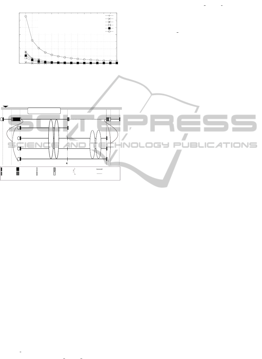
We show an experiment to demonstrate the latency

tolerance in the Microgrid using MGSim. We cre-

ate few families with instructions from different cat-

egories explained below. The extra cycles consumed

by long latency operations in these families are shown

in ﬁg. 1. The x-axis shows the window size used

during the execution and the y-axis shows the cycles

taken by the long latency operations and are normal-

ized per instruction. The normalization is subtracting

the number of instructions from total latency, divided

by the number of instructions. In this experiment we

show three families for variable latency operations i.e.

short, medium and large. The idea is to show that

variable latency operations are difﬁcult to simulate,

and changing a single parameter affects the through-

put and hence the extra cycles consumed. The details

of the created families is given below:

• One nop instruction per thread: An empty thread

has one nop (no-operation), because the fetch

stage needs to know when to terminate a thread.

When only one thread is active, it has an overhead

to schedule instructions. But as the window size

increases the latency is reducing. After window

size 8, we have a full pipeline and therefore, the

latency is close to 0.

• Single-cycle-latency instructions: When only one

thread is active, we have the overhead of creating

and cleaning thread, but as soon as the window

size is 2 or more the extra latency is reduced to

zero.

• Fixed-latency instructions: When only one thread

is active, it has the latency of 8 cycles. 6 cycles

are taken in the pipeline and extra 2 cycles in-

clude the overhead of creation and cleanup of the

thread. When the number of threads increases this

extra latency is reducing. After 8 or more threads

are active, the pipeline becomes full and the extra

latency is close to 0.

• Variable-latency instructions (short): We count

the time for creating a family on a single core. The

communication is only between the parent core

and the core in the delegated place, therefore the

latency of allocate, create and sync is considered

as short variable latency instructions.

• Variable-latency instructions (medium): We count

the time for creating a family on four cores. The

communication is between the parent core and

the four cores in the delegated place. The cycles

taken by allocate, create and sync is considered as

medium variable latency instructions.

• Variable-latency instructions (large): We count

the time for creating a family on 64 cores. Since a

large number of cores are used for the distribution

of threads, therefore the latency of allocate, create

and sync is considered as large variable latency

instructions.

Signature-basedHigh-levelSimulationofMicrothreadedMany-coreArchitectures

511

0 5 10 15

Cycles dedicated to non-local latencies

normalized per instruction

= (total latency - nr of instructions) / (nr of instructions)

Concurrent threads

Latency tolerance

for families of 100 threads

1 nop per thread

1-cycle instructions only

Fixed-latency instructions (FPU)

Variable-latency instructions (short)

Variable-latency instructions (medium)

Variable-latency instructions (large)

Figure 1: Latency tolerance exhibited by different types of

families, where every family creates 100 threads with dif-

ferent types of instructions and hence demonstrate different

latency tolerance.

0 10 20 245 455 460 470

Sig(5,5,5)

Clock

A dependent family of threads

Thread executing

Thread waiting

Start thread

End thread

Read shared

Write shared

Allocate family

Create family

Sync family

Release family

Wakeup event

Read/write by parent

Interleaving

Sig(x,y,z) = Signature(AIS_SINGLE_LATENCY, AIS_FIXED_LATENCY, AIS_VARIABLE_LATENCY)

Sig(5,0,0)

Sig(10,0,0)

Thread ID

Sig(5,5,5)

Sig(10,5,5)

Sig(5,5,10)

Sig(5,10,5)

Sig(5,0,0)

Sig(0,0,5)

Sig(0,5,0)

Fixed latency factor = 2

Variable latency factor = 6

Fixed latency factor = 8

Variable latency factor = 33

Original: (5 x 5) + (5 x 5) + (5x5) = 75

Adapted: (5x5) + (5x5x2) + (5x5x6) = 225

Figure 2: Abstraction of instruction execution using signa-

tures with the latency factor model.

5 HIGH-LEVEL SIMULATION OF

FINE-GRAINED LATENCY

TOLERANCE

The abstracted instruction execution in case of signa-

ture is shown in ﬁg. 2. We analyze threads based on

the indices of the signature i.e. we look for the thread

with minimum single latency, minimum ﬁxed latency

and minimum variable latency instructions, making

sure that instructions of zero are not counted as the

minimum. The minimum number of instructions are

multiplied with the number of active threads and the

latency factor (c.f. section 5.1) in order to compute

the warp time. The active threads are the number of

threads which have instructions in any of the three cat-

egories of AIS. The simulation time is then advanced

and the numbers in the signatures are reduced as per

the calculated minimum number of instructions. This

process is summarized into three steps:

1. Calculate time warp:

Time warp = min(Sig[0]

(1..n)

) × n

+min(Sig[1]

(1..n)

) × f ixed latency f actor × n

+min(Sig[2]

(1..n)

) × variable latency f actor × n

; where n

is the number of active threads such that

sig[x] > 0 with x 0, 1 or 2 and min(Sig[x]

(1..n)

) > 0.

2. Advance simulated time:

Clock+ = Time warp

3. Reduce workload of all active threads:

Sig[0]

(1..n)

− = min(Sig[0])&

Sig[1]

(1..n)

− = min(Sig[1])&

Sig[2]

(1..n)

− = min(Sig[2])

These steps continue to execute until the signa-

tures become of the form Sig(0, 0, 0), in which case

the event of the thread is completed and the applica-

tion model is notiﬁed to send the next event.

5.1 The latency hiding factor

The latency factor model gives approximate numbers

that can be used to adapt the throughput of the pro-

gram based on the type of instructions executing and

the number of threads in the pipeline. It is derived

from the experiment explained in section 4. The la-

tency hiding factor model is given in table 2. With

one active thread we have a high latency factor for

ﬁxed and variable instructions. But as the number of

active threads increases, the latency hiding factor de-

creases. With 8 active threads the latency factor for

ﬁxed latency instructions is 1. The variable latency

factor can also be 1, depending on the distribution of

an application on the Microgrid and the frequency of

having a full pipeline during the execution. Given that

our benchmarks are not very well distributed, we as-

sume that the variable latency factor when there are 8

or more active threads is 2.

With 8 or more active threads the throughput of

the program is similar to One-IPC HLSim, because

there are always enough active threads during the

computation of warp time and therefore the through-

put is always computed as one cycle per instruction

i.e. the assumption of One-IPC HLSim. The pri-

mary contribution of the latency factor model is that

it adapts the throughput of the program as per the dy-

namic number of active threads during the execution

of the program.

6 RESULTS

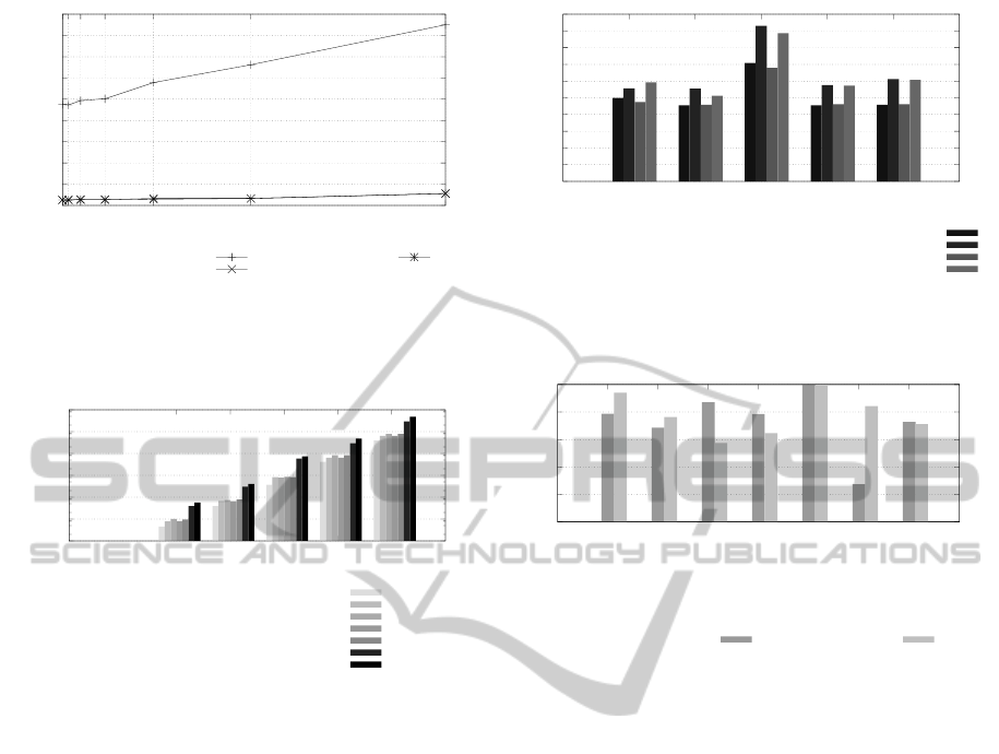
6.1 Ratio in simulated time

In order to see the difference in simulated time be-

tween Signature-based HLSim and MGSim, we com-

pute the ratio of cycles in both simulators and com-

pare this with the same ratio using One-IPC HLSim.

SIMULTECH2014-4thInternationalConferenceonSimulationandModelingMethodologies,Technologiesand

Applications

512

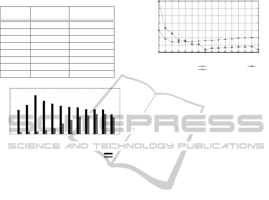
Table 2: The latency factor model.

Active Fixed latency Variable latency

threads factor factor

1 8 33

2 4 16

3 3 11

4 3 7

5 2 6

6 2 4

7 2 3

8 or more 1 2

128

256

512

1024

2048

4096

8192

16384

32768

65536

Ratio (simulated time)

FFT data size

(Cycles in MGSim/Cycles in One-IPC HLSim)

(Cycles in MGSim/Cycles in Signature-based HLSim)

Figure 3: Ratio in simulated time of FFT using different

data sizes and executing on 64 simulated cores.

These ratios are shown in ﬁg. 3 for different data

sizes. A value close to 1 means the simulators pre-

dict the same execution time.

The Signature-based HLSim is always more accu-

rate than One-IPC HLSim. The difference is more

signiﬁcant with smaller data sizes, where there are

fewer threads per core. The difference is no more than

a factor of 3 for data sizes less than 512 over 64 cores,

which gives less than 4 threads per core. In this range

the dynamic adaptation of the simulator, where the

number of threads moderates the cost of long latency

operations shows the best accuracy. As the number

of threads increases the latency tolerance factor is re-

duced and the results of the two simulators converge

and both are about a factor of 10 out.

Two potential factors may contribute to the diver-

gence between MGSim and HLSim. The ﬁrst is that

we do not limit the number of threads based on regis-

ter ﬁle size, so in this application we overestimate the

number of threads. Secondly, we are not considering

the differences in latency due to accessing different

levels of caches.

50000

100000

150000

200000

250000

300000

350000

400000

1 2 3 4 5 6 7 8 9 10 11 12 13 14 15 16

Simulated time (Cycles)

Window size

MGSim

One-IPC HLSim

Signature-based HLSim

Figure 4: The effect of changing the window size on the

execution of FFT of data size 2

executing on 2

cores.

6.2 The effect of window size on

simulated time

The simulated time of One-IPC HLSim, Signature-

based HLSim and MGSim in executing FFT of size

on 2

cores based on the window size in the range

of 1 to 16 is shown in ﬁg. 4. We can see that the sim-

ulated time in One-IPC HLSim remain a straight line,

because the throughput is not adapted. In Signature-

based HLSim the simulated time is not the same as

in MGSim, but the behavior of simulated time based

on different number of active threads is similar in both

simulators. In both simulators, when there is only one

active thread, the simulated time is very high, but as

the number of threads increases the simulated time

starts to decrease because of latency tolerance. In ei-

ther case, the throughput as one instruction per cycle

is not achieved, because of the overhead of concur-

rency and long latency operations. This is an impor-

tant contribution of the Signature-based HLSim, as

based on the number of active threads and number of

instructions it has adapted the throughput. We do not

see this adaptation when there are always more than 8

active threads, but this experiment shows that the sim-

ulation technique presented in this paper improves the

accuracy of the high-level simulator.

6.3 Simulation time

We execute a Mandelbrot set approximation of dif-

ferent complex plane sizes and different number of

cores. FFT is memory-bound and Mandelbrot is

compute-bound. Which means that Mandelbrot is

more accurate in Signature-based HLSim than FFT.

Since we are not simulating memory operations in

Signature-based HLSim, there is no effect on the sim-

ulation time. We show the simulation time of Mandel-

brot to give a different application for evaluation. We

show two experiments of simulation time; in the ﬁrst

Signature-basedHigh-levelSimulationofMicrothreadedMany-coreArchitectures

513

500

1000

1500

2000

2500

3000

3500

4000

4500

5000

1 2 4 8 16 32 64

Simulation time (Seconds)

Number of cores

MGSim

One-IPC HLSim

Signature-based HLSim

Figure 5: Simulation time in the execution of Mandelbrot

set (Complex Plane: 1000 × 1000) on different number

of cores of One-IPC HLSim, Signature-based HLSim and

MGSim.

0.01

0.1

100

1000

10000

10x10 31x31 100x100 316x316 1000x1000

Simulation time (Seconds)

Size of complex plane

Front-end HLSim (window size 256)

One-IPC HLSim (core 1)

One-IPC HLSim (cores 64)

Signature-based HLSim (core 1)

Signature-based HLSim (cores 64)

MGSim (core 1)

MGSim (cores 64)

Figure 6: Simulation time of Front-end HLSim, One-IPC

HLSim, Signature-based HLSim and MGSim in computing

Mandelbrot of different complex plane sizes.

experiment we execute a particular complex plane

on different number of cores. The simulation time

(i.e. simulation speed) of Mandelbrot approximation

set of complex plane size 1000 × 1000 across a range

of simulated cores is given in ﬁg. 5. The x-axis shows

the number of simulated cores and the y-axis shows

the simulation time in the range of program execu-

tion. We can see that the simulation time of Signature-

based HLSim is the same as One-IPC HLSim, indi-

cating that we can achieve accuracy without affecting

the simulation speed.

In the second experiment we execute a complex

plane of different sizes using selected number of

cores. We show this experiment in different simula-

tors in ﬁg. 6. The x-axis shows the size of the com-

plex plane and y-axis shows the simulation time in the

range of program execution.

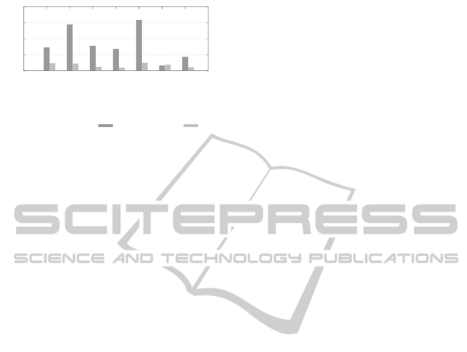
In order to see the speedup in simulation time

by Signature-based HLSim compared to MGSim, we

compute the ratio in simulation time of simulating 1

and 64 cores in MGSim divided by the simulation

time in simulating 1 and 64 cores in Signature-based

HLSim respectively. This ratio is shown in ﬁg. 7. The

ratio for Signature-based HLSim against MGSim re-

10x10 31x31 100x100 316x316 1000x1000

Ratio in simulation time

Size of complex plane

[Seconds in MGSim/Seconds in One-IPC HLSim] (core 1)

[Seconds in MGSim/Seconds in One-IPC HLSim] (cores64)

[Seconds in MGSim/Seconds in Signature-based HLSim] (core 1)

[Seconds in MGSim/Seconds in Signature-based HLSim] (cores64)

Figure 7: Ratio in simulation time of One-IPC HLSim

and Signature-based HLSim against MGSim in computing

Mandelbrot of different complex plane sizes.

0.2

0.4

0.6

0.8

GOL(Torus)

GOL(Grids)

FFT

LMK7

Mandelbrot

MatrixMultiply

Smooth

IPC

Signature-based HLSim MGSim

Figure 8: Average IPC achieved by MGSim and Signature-

based HLSim.

mains exactly the same as One-IPC HLSim demon-

strating that the simulation speed is not affected.

6.4 IPC - Simulation accuracy

Instructions Per Cycle (IPC) shows the efﬁciency

(Not performance, as that also depends on the clock

frequency) of the architecture. For each core the IPC

should be as close to the number of instructions the ar-

chitecture is capable of issuing in each cycle. In case

of the Microgrid, with single issue, the IPC of each

core should be as close to 1 as possible. However, for

c cores, the overall IPC may be up to c, i.e. each core

may issue 1 instruction per cycle. We can also mea-

sure the average IPC, i.e. sum the IPC of c cores di-

vided by c. We show the IPC achieved by HLSim and

MGSim in ﬁg. 8. We can see that in FFT, LMK7 and

Mandelbrot we see a closer IPC by Signature-based

HLSim to MGSim. In others the IPC is not closer

by different simulators, because of the different num-

ber of large latency operations and also because of the

dynamic state of the system.

SIMULTECH2014-4thInternationalConferenceonSimulationandModelingMethodologies,Technologiesand

Applications

514

500

1000

1500

2000

GOL(Torus)

GOL(Grids)

FFT

LMK7

Mandelbrot

MatrixMultiply

Smooth

KIPS

Signature-based HLSim MGSim

Figure 9: Average IPS achieved by MGSim and Signature-

based HLSim.

6.5 IPS - Simulation speed

Instructions per second (IPS) is used to measure the

basic performance of an architecture, as we can mea-

sure the simulated instructions per second using a

known contemporary processor. The average IPS (av-

erage across all the cores) achieved by Signature-

based HLSim and MGSim is shown in ﬁg. 9. We

can see that the IPS of MGSim is approximately 100

KIPS, and the IPS of Signature-based HLSim is ap-

proximately 1 MIPS. Different simulators used in in-

dustry and academia with their simulation speed in

terms of IPS are: COTSon (Argollo et al., 2009)

executes at 750KIPS, SimpleScalar (Austin et al.,

2002) executes at 150KIPS, Interval simulator (Carl-

son et al., 2011) executes at 350KIPS and Sesame (Er-

bas et al., 2007) executes at 300KIPS. MGSim (Bou-

sias et al., 2009) executes at 100KIPS. Compared to

the IPS of these simulators the IPS of HLSim is very

promising. It should be noted that the IPS of sim-

ulation frameworks given above are simulating only

few number of cores on the chip. In MGSim and

HLSim we have simulated 128 cores on a single chip.

Given this large number of simulated cores on a chip,

1 MIPS indicates a high simulation speed.

7 CONCLUSION

Signatures are introduced to estimate the number of

instructions in abstracted categories of basic blocks.

These signatures are then used to model the dynamic

adaptation of the program based on the currently ac-

tive threads per core. In this paper, we have simu-

lated load operation as a variable latency operation

and have treated store operation as single latency op-

eration. Also we have ignored the simulation of reg-

ister ﬁles in HLSim. In the future work we would

like to simulate store and register ﬁles in HLSim and

analyze if the accuracy can further be improved.

REFERENCES

Argollo, E., Falc

on, A., Faraboschi, P., Monchiero, M., and

Ortega, D. (2009). Cotson: infrastructure for full sys-

tem simulation. SIGOPS Oper. Syst. Rev., 43(1):52–

61.

Austin, T., Larson, E., and Ernst, D. (2002). SimpleScalar:

An Infrastructure for Computer System Modeling.

Computer, 35(2):59–67.

Bammi, J. R., Kruijtzer, W., Lavagno, L., Harcourt, E., and

Lazarescu, M. T. (2000). Software performance es-

timation strategies in a system-level design tool. In

Proceedings of the eighth international workshop on

Hardware/software codesign, CODES ’00, pages 82–

86, New York, NY, USA. ACM.

Bernard, T. A. M., Grelck, C., Hicks, M. A., Jesshope,

C. R., and Poss, R. (2011). Resource-agnostic pro-

gramming for many-core microgrids. In Proceed-

ings of the 2010 conference on Parallel processing,

Euro-Par 2010, pages 109–116, Berlin, Heidelberg.

Springer-Verlag.

Bousias, K., Guang, L., Jesshope, C. R., and Lankamp,

M. (2009). Implementation and evaluation of a mi-

crothread architecture. J. Syst. Archit., 55:149–161.

Carlson, T. E., Heirman, W., and Eeckhout, L. (2011).

Sniper: exploring the level of abstraction for scalable

and accurate parallel multi-core simulation. In Pro-

ceedings of 2011 International Conference for High

Performance Computing, Networking, Storage and

Analysis, SC ’11, pages 52:1–52:12, New York, NY,

USA. ACM.

Corporation, D. E. (1992). Alpha Architecture Handbook.

Eeckhout, L., Nussbaum, S., Smith, J. E., and Bosschere,

K. D. (2003). Statistical simulation: Adding efﬁ-

ciency to the computer designer’s toolbox. IEEE Mi-

cro, 23:26–38.

Erbas, C., Pimentel, A. D., Thompson, M., and Polstra,

S. (2007). A framework for system-level modeling

and simulation of embedded systems architectures.

EURASIP J. Embedded Syst., 2007:2–2.

Giusto, P., Martin, G., and Harcourt, E. (2001). Reliable es-

timation of execution time of embedded software. In

Proceedings of the conference on Design, automation

and test in Europe, DATE ’01, pages 580–589, Piscat-

away, NJ, USA. IEEE Press.

Jesshope, C. (2008). A model for the design and pro-

gramming of multi-cores. Advances in Parallel Com-

puting, High Performance Computing and Grids in

Action(16):37–55.

Jesshope, C., Lankamp, M., and Zhang, L. (2009). The

implementation of an svp many-core processor and

the evaluation of its memory architecture. SIGARCH

Comput. Archit. News, 37:38–45.

Jesshope, C. R. (2004). Microgrids - the exploitation of

massive on-chip concurrency. In Grandinetti, L., ed-

itor, High Performance Computing Workshop, vol-

ume 14 of Advances in Parallel Computing, pages

203–223. Elsevier.

Lankamp, M., Poss, R., Yang, Q., Fu, J., Uddin, I., and

Jesshope, C. R. (2013). MGSim - Simulation tools

Signature-basedHigh-levelSimulationofMicrothreadedMany-coreArchitectures

515

for multi-core processor architectures. Technical Re-

port arXiv:1302.1390v1 [cs.AR], University of Ams-

terdam.

Poss, R. (2012). SL—a “quick and dirty” but working in-

termediate language for SVP systems. Technical Re-

port arXiv:1208.4572v1 [cs.PL], University of Ams-

terdam.

Uddin, I. (2013). Microgrid - The microthreaded many-core

architecture. Technical report, University of Amster-

dam. arXiv Technical report.

Uddin, I., Jesshope, C. R., van Tol, M. W., and Poss, R.

(2012). Collecting signatures to model latency toler-

ance in high-level simulations of microthreaded cores.

In Proceedings of the 2012 Workshop on Rapid Sim-

ulation and Performance Evaluation: Methods and

Tools, RAPIDO ’12, pages 1–8, New York, NY, USA.

ACM.

Uddin, I., van Tol, M. W., and Jesshope, C. R. (2011). High-

level simulation of SVP many-core systems. Parallel

Processing Letters, 21(4):413–438.

SIMULTECH2014-4thInternationalConferenceonSimulationandModelingMethodologies,Technologiesand

Applications

516