
General Road Detection Algorithm
A Computational Improvement
Bruno Ricaud, Bogdan Stanciulescu and Amaury Breheret
Centre de Robotique, Mines ParisTech, 60 Boulevard St Michel, 75006 Paris, France
Keywords:
Vanishing Point, Gabor, Image Processing, Offroad, Computation, Autonomous Driving.
Abstract:
This article proposes a method improving Kong et al. algorithm called Locally Adaptive Soft-Voting (LASV)
algorithm described in ”General road detection from a single image”. This algorithm aims to detect and
segment road in structured and unstructured environments. Evaluation of our method over different images
datasets shows that it is speeded up by up to 32 times and precision is improved by up to 28% compared to the
original method. This enables our method to come closer the real time requirements.
1 INTRODUCTION
This work focuses on road detection and reconstruc-
tion in semi-natural environment, such as dirt roads,
natural pathways or country roads which are hard to
follow. Our aim is in providing the driver with a help-
ful assistance and quantify the difficult conditions that
an unprepared road brings. Subsequently, in the fu-
ture, we plan to apply this kind of assistance to au-
tonomous robots navigation. To this aim, we plan to
use monocular ground shape detection, using the wa-
tersheds algorithm (Vincent and Soille, 1991; Mar-
cotegui and Beucher, 2005).
In road detection applications the vanishing point
plays a central role, for various reasons but mainly for
the size reduction of the search area. This reduction
usually provides faster computation and better perfor-
Figure 1: Vanishing point detection in all type of environ-
ment, although without any lane marking.
mance with less false positives. To create a complete
algorithm for road detection we started with vanish-
ing point detection. Kong et al. algorithm is very
effective on non-urban roads. One big challenge with
this algorithm resides in its computational time which
is very long. This is why we have improved its per-
formances and tested the resulting method. Indeed in
our application we plan to use real time camera. In
this paper, an important part of our contribution is to
speed it up to meet the real-time requirements. Thus,
our method consists of essentially three contributions
over the original algorithm. First we have changed
the image transformation, second we have highly in-
creased the computation speed, and finally we have
improved the original algorithm precision.
2 VANISHING POINT
2.1 Generalities
When surveying the state of the art, we wanted
to test algorithms for vanishing point detection.
A road, curved or straight, in urban or non-urban
environment, can be modelled as two straight lines
which converge on the horizon line. The convergence
point is the vanishing point. This point answers three
main interrogations : Where is the ground? Where is
the sky? Where the road goes?
Different articles (Tardif, 2009; Nieto and Salgado,
2011) and algorithms exists, this problematic is
known for few years (Rother, 2002) but Kong’s
825
Ricaud B., Stanciulescu B. and Breheret A..
General Road Detection Algorithm - A Computational Improvement.
DOI: 10.5220/0004935208250830
In Proceedings of the 3rd International Conference on Pattern Recognition Applications and Methods (USA-2014), pages 825-830
ISBN: 978-989-758-018-5
Copyright
c
2014 SCITEPRESS (Science and Technology Publications, Lda.)

Figure 2: Vanishing Point Detection.
Top row: (1) Starting image. (2) Creation of the edge image. (3) Finding of textures orientations image with Gabor filter.
(4) Thresholding of textures orientations map and creation of the confidence map. Bottom row: (5) Candidate pixels vote.
(6) Creation of the vote map (7) Election of the most popular pixel of the vote map (8) The vanishing point has been found
[PINK], it will be compared to the groundtruth [WHITE].
Locally Adaptive Soft-Voting (LASV) algorithm
is the most effective in the spectrum of our appli-
cation. Indeed LASV is designed to detect roads
and pathways in every type of environment(Fig.1)
using Gabor filter(Dunn et al., 1995) whereas other
methods usually use Hough filter(Maitre, 1985) to
detect lanes marking or road borders and are limited
to urban situation. In Kong et al. article an entire road
segmentation is proposed. For our work we aimed
only for vanishing point detection which provides us
with all needed information.
2.2 LASV
To summarize LASV we have extracted two step by
step tables from (Kong et al., 2010) and we have
rewritten them in the following I. and II. table sec-
tions. For our method we focus only on the first part
of the algorithm which handles vanishing point detec-
tion (I. Locally adaptive soft-voting (LASV) scheme).
I. Locally adaptive soft-voting (LASV) scheme
(Fig.2)
1) For each pixel of the input image, com-
pute the confidence in its texture orientation esti-
mation(computed with the Gabor Filter).(Fig.2.3)
2) Normalize the confidence to the range of 0
to 1, and only keep as voters the pixels whose con-
fidence is larger than 0.3(which has been found
empirically).(Fig.2.4)
3) Only the pixels in the top 90% portion of
the image are selected as vanishing point candi-
dates.
4) Create a local voting region R
v
, for each
vanishing point candidate and only the voters
within R
v
vote for it.
5) Vote for each vanishing point candidate
(Fig.2.6) based on :
Vote(P, V ) =
(
1
1+
γd(P,V)
2
, if γ ≥
5
1+2d(P,V)
0 , γ even
(1)
6) The pixel which receives the largest voting
score is selected as the initial vanishing point.
II. Vanishing point constrained road border detection
1) Starting from the initially estimated van-
ishing point vp
0
, construct a set of evenly dis-
tributed imaginary rays.
2) For each ray, compute two measures, i.e.,
OCR
1
and color difference.
3) Select the ray as the first road border if it
satisfies the following two conditions:
3.a) It maximizes the following criterion,
ie., :
b = arg
i
max
di f f (A1, A2)x
i+1
∑
j=i−1
OCR
j
(2)
3.b) Its length is bigger than
1
3
of the im-
age height.
1
Orientation Constitency Ratio : l is a line constituted by a
set of oriented points. For each point, if the angle between point
orientation and direction line is less than a threshold, the point has
a consistent line orientation. OCR is defined as the ratio between
the number of consistent points and the number of line points.
ICPRAM2014-InternationalConferenceonPatternRecognitionApplicationsandMethods
826

4) Update the vanishing point estimation:
4.a) Regularly sample some points (with a
four-pixel step) on the first road border denoted
p
s
.
4.b) Through each point of p
s
, respec-
tively construct a set of 29 evenly distributed rays
(spaced by 5
◦
, whose orientation from the hori-
zon is more than 20
◦
, and less than 180
◦
) for each
point of p
s
, denoted as L
s
4.c) From each L
s
, find a subset of n rays
such that their OCRs rank top n among the 29
rays.
4.d) The new vanishing point vp
1
is se-
lected from p
s
as the one which maximizes the
sum of the top n OCRs
1
.
5) Starting from vp
1
, detect the second road
border in a similar way as the first border, with a
constraint that the angle between the road borders
is larger than 20
◦
.
3 OUR APPROACH
Our interest in LASV (Kong et al., 2010) is motivated
by the possibility of using it as a pre-segmentation for
our application. Our implementation aims to work on
a vehicle platform equipped with a 30 FPS camera.
This is why we needed to accelerate its computation
to meet the real time requirements.
We tested this algorithm on several datasets (Geiger
et al., 2012; Kong et al., 2010; Leskovec et al.,
2008), in our case this algorithm will be used with
continuous capture. This is why we have tried to
improve this method on datasets using successive
frames instead of random environment pictures
datasets like the ones used by Kong.
The original code was written in MATLAB by Kong.
During the initial tests, the original implementation
required a computation time of 18 seconds per image.
Our optimisation is mainly concentrated on step
I.3) of the original algorithm. Our improvements
were done in the same environment in several steps.
We have benchmarked each evolution to justify its
purpose.
3.1 Methods
For all methods, we have reduced image size down
to 240 pixels height and 180 pixels width, just like
the original algorithm does. The (Fig.3) illustrates
subsequent methods (it shows an asphalt road, indeed
this algorithm worked on unmarked and marked
road).
Method I Temporal Dependence
a) For first image, computation of vanishing point
research is done on the complete image.
b) For subsequent images, the best vanishing point
candidate is only selected from a 10% by 10% image
size zone around the coordinates of the vanishing
point found previously.
The 10% by 10% range is explained by the fact that
the image will not move much between two frames,
considering camera preset of 30 FPS. The length of
10% image size has been found empirically.
Method II Reset
a) The temporal method is used but at every 10
frames we do a complete image computation.
Method III Size Reduction
a) Image size is decreased by half before doing
the complete image computation. This operation is
repeated on every images.
Method IV Temporal + Size Reduction + Reset
a) Image size is decreased by half before computing
the vanishing point research.
b) For first image, computation of vanishing point
research is done on the complete image.
c) For subsequent images, the best vanishing point
candidate is only selected from a 10% by 10% image
size zone around the coordinates of the vanishing
point previously found in order to refine the vanishing
point position.
d) Every 10 images, the computation is done on the
complete image.
Method V Downsampling
a) Image size is decreased by half before computing
the vanishing point research.
b) Image size is then increased and the best vanishing
point candidate is only selected from a 10% by 10%
image size zone around the coordinates of the vanish-
ing point found previously on the same but smaller
image in order to refine the vanishing point position.
c) These operations are done on every image.
Method VI Temporal + Downsampling + Reset
a) Image size is decreased by half before computing
the vanishing point research.
b) Image size is then increased and the best vanishing
point candidate is only selected from a 10% by 10%
image size zone around the coordinates of the vanish-
ing point previously found on the same but smaller
image in order to refine the vanishing point position.
c) The following image size is decreased by a ratio
GeneralRoadDetectionAlgorithm-AComputationalImprovement
827
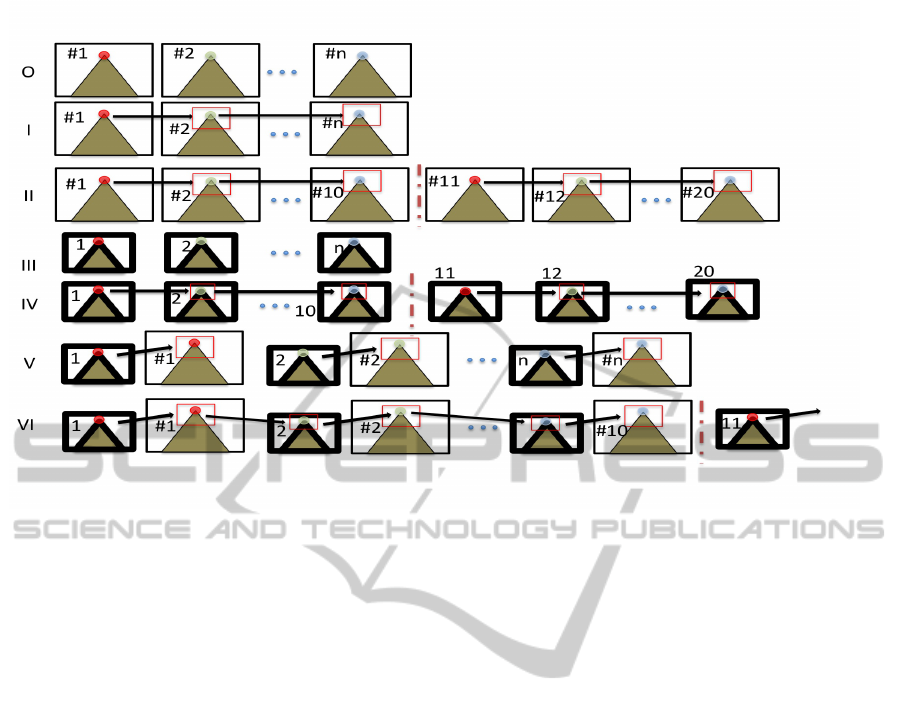
Figure 3: Methods schematic.
O, Original Method : Complete image computation; I, Method I : Arrows show temporal dependency; II, Method II : Dashed
bar shows the reset every ten images; III, Method III : Smaller image show image size reduction; ...
before computing the vanishing point only on a
10% by 10% image size zone around the coordinates
of the vanishing point found in step b).
d) Image size is then increased and the computation is
done only on a 10% by 10% image size zone around
the coordinates of the vanishing point previously
found in order to refine the vanishing point position.
e) Every 10 images, the computation is done on the
complete reduced image.
We also wanted to see the differences in perfor-
mance between gradient images and edge images.
We have compared methods using pre-processed
Prewitt images with same methods using in turn
pre-processed Canny images.
In order to evaluate the methods we have manually
labelled a dataset with the ground-truth location of
vanishing points. We used raw data from the Kitti
Road dataset (Geiger et al., 2012).
We used two datasets for benchmarking, one also
used by LASV author was already labelled with
vanishing points, the second has been labelled by
our own. All images were used with the resolution
180x240 following author’s strategy.
The LASV dataset is composed of 1003 independent
images and taken in different environments. This
dataset is difficult for algorithm but useful because
most of these pictures are missing lane marking and
asphalt which make path harder to detect. We used
this dataset only on original method and method V.
Indeed all temporal method aren’t able to be used on
independent images datasets.
The second dataset is a 250 images dataset which are
following each other. Ground truth has been labelled
using different students estimation. After explaining
the vanishing point theory, each student has labelled
vanishing points in the datasets. Following these
labelling period, we have taken every labelled dataset
to compute the average coordinates of vanishing
points in each image. This average coordinates are
considered as ground truth.
The computation of the local error consists of com-
puting the Euclidean distance between location of
the computed vanishing point and its ground-truth
location. Global error of each method is the average
of all local errors.
This comparison allowed us to created 3 classifica-
tions : precision classification, speed classification
and speed + precision classification.
3.2 Results
Benchmarking shows a gradual improvement in
methods result (Tab.3). From original method to
method I we wanted to speed-up the computation by
adding a temporal dependency. The temporal depen-
dency provided a small speed-up (Tab.1) but also a
big loss in precision (Tab.2). A precision of 65.2%
on an image of 180x240 is extremely low, with tem-
poral dependency, vanishing point detection is often
lost. This explains method II which was created to de-
crease the temporal dependency errors. We changed
ICPRAM2014-InternationalConferenceonPatternRecognitionApplicationsandMethods
828
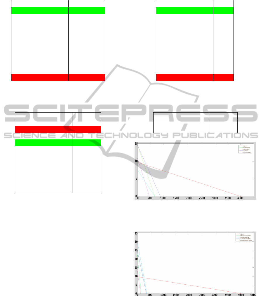
Table 1: Speed Classification.
Method Speed (FPS)
Method IV (gradient) 1.96
Method IV (edge) 1.66
Method VI (gradient) 0.71
Method VI (edge) 0.66
Method III (gradient) 0.53
Method I 0.42
Method V (gradient) 0.367
Method III (edge) 0.366
Method V (edge) 0.27
Method II 0.21
Original 0.06
Table 2: Precision Classification. Error is the average Eu-
clidian distance between groundtruth and found vanishing
point on all the dataset. Precision is this error compared to
half the image size.
Method Precision
Method V (gradient) 94.92%
Original 93.50%
Method III (gradient) 92.66%
Method IV (gradient) 91.12%
Method V (edge) 90.28%
Method III (edge) 90.22%
Method IV (edge) 84.80%
Method VI (gradient) 83.26%
Method VI (edge) 79.74%
Method II 78.06%
Method I 30.41%
dependency to be used only on intervals (10 images).
Indeed this method shows us that smaller steps give
smaller errors (Tab.2) but a longer computation time
(Tab.1). The method III followed the original method
where images size is yet decreased. We wanted to
see to which point, images size reduction would even
bring enough information to be useful. This method
revealed to be very effective in both speed and preci-
sion (Tab.3).
In method IV we used image reduction and tem-
poral dependency together which shows us very in-
teresting results. Speed had been improved a lot but,
a light loss was also present. This is why we have
continued to search method which can bring speed-
up and precision maintenance. In method V, we used
the downsampling method, inspired by the FPDW
method (Dollar et al., 2010). We created this method
thinking that dependency between two sizes of a same
image could bring us more precision (Tab.2) without
wasting too much time (Tab.1). This has been con-
firmed with benchmarks (Tab.3). Method VI was in-
cluded to show that temporal dependency continues
to provide a speed-up but also loses precision (Tab.2)
Table 3: Speed * Precision Classification.
Method #
Method IV (gradient) 1.786
Method IV (edge) 1.41
Method VI (gradient) 0.591
Method VI (edge) 0.526
Method III (gradient) 0,491
Method V (gradient) 0,348
Method III (edge) 0,33
Method V (edge) 0,244
Method II 0,164
Method I 0,143
Original 0,05
Table 4: Precision Classification on ENS Dataset (1003 im-
ages in difficult situations. Error is the average Euclidian
distance between groundtruth and found vanishing point on
all the dataset.
Method Precision
Original 88.46%
Method V (gradient) 88.01%
Figure 4: Global Error/ Computation time on 250 images:
(red) Original (purple) Method III [gradient] (cyan) Method
V [gradient] (green) Method III [edge] (blue) Method V
[edge].
Figure 5: Global Error/ Computation time on 250 im-
ages: (red) Original (Pink) Method IV [gradient] (dark
blue) Method VI [gradient] (green) Method IV [edge] (clear
blue) Method VI [edge].
worse than method II, which shows that too much de-
pendency decreases precision.
Results show that new methods bring speed
improvements (fig.5) and precision improvements
GeneralRoadDetectionAlgorithm-AComputationalImprovement
829
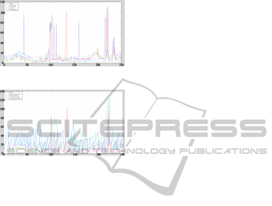
Figure 6: Local errors on each image: (red) Original
(purple) Method III [gradient] (cyan) Method V [gradient]
(green) Method III [edge] (blue) Method V [edge].
Figure 7: Local errors on each image: (red) Original (pink)
Method IV [gradient] (dark blue) Method VI [gradient]
(green) Method IV [edge] (clear blue) Method VI [edge].
(fig.4). Results also show that gradient images based
methods are faster and more accurate due to the addi-
tional information brought by gradient images com-
pared to edge images based methods. The method
which is the most efficient is Method IV (Temporal +
Size Reduction + Reset). This method does not bring
the best precision but is the fastest and is not quite far
from original version concerning precision.
4 CONCLUSIONS AND FUTURE
WORKS
The obtained results show the entire potential that our
improved version of the LASV could have for the pre-
segmentation stage. We have improved its precision
and speed it up by more than 32 times to come closer
to the real time requirements (30 FPS), indeed our
improvements are around 2FPS on Matlab compared
to the 0.06 FPS of the original LASV. Moreover, our
method is almost as precise as the original algorithm.
We now plan to create an embedded version of this
code and expect to see an additional speed-up com-
pared to the MATLAB implementation. The results
would be highly increased and even closer to real time
requirements.
We plan to use this pre-segmentation as an aid
for road segmentation using watersheds (Vincent and
Soille, 1991; Marcotegui and Beucher, 2005) employ-
ing this method to limit the region of interest area and
reduce computation time.
REFERENCES
Dollar, P., Belongie, S., and Perona, P. (2010). The Fastest
Pedestrian Detector in the West. Procedings of the
British Machine Vision Conference 2010, pages 68.1–
68.11.
Dunn, D., Higgins, W. E., and Member, S. (1995). Optimal
Gabor Filters for Texture Segmentation. 4(7).
Geiger, A., Lenz, P., and Urtasun, R. (2012). Are we ready
for autonomous driving? the kitti vision benchmark
suite. In Conference on Computer Vision and Pattern
Recognition (CVPR).
Kong, H., Audibert, J.-Y., and Ponce, J. (2010). General
road detection from a single image. IEEE transac-
tions on image processing : a publication of the IEEE
Signal Processing Society, 19(8):2211–20.
Leskovec, J., Lang, K. J., Dasgupta, A., and Mahoney,
M. W. (2008). Community structure in large net-
works: Natural cluster sizes and the absence of large
well-defined clusters. CoRR, abs/0810.1355.
Maitre, L. (1985). Un panorama de la transformation de
Hough. 2:305–317.
Marcotegui, B. and Beucher, S. (2005). FAST IM-
PLEMENTATION OF WATERFALL BASED ON
GRAPHS.
Nieto, M. and Salgado, L. (2011). Simultaneous estima-
tion of vanishing points and their converging lines us-
ing the {EM} algorithm. Pattern Recognition Letters,
32(14):1691 – 1700.
Rother, C. (2002). A new Approach to Vanishing Point
Detection in Architectural Environments. (January
2002):1–17.
Tardif, J.-P. (2009). Non-iterative approach for fast and
accurate vanishing point detection. 2009 IEEE
12th International Conference on Computer Vision,
(Iccv):1250–1257.
Vincent, L. and Soille, P. (1991). Watersheds in Digital
Spaces : An Efficient Algorithm Based on Immersion
Simulations. IEEE transactions on pattern analysis
and . . . .
ICPRAM2014-InternationalConferenceonPatternRecognitionApplicationsandMethods
830
