Initialization Framework for Latent Variable Models
Heydar Maboudi Afkham, Carl Henrik Ek and Stefan Carlsson
Computer Vision and Active Preception Lab., KTH, Stockholm, Sweden
Keywords:
Latent Variable Models, Clustering, Classification, Localization.
Abstract:
In this paper, we discuss the properties of a class of latent variable models that assumes each labeled sample is
associated with set of different features, with no prior knowledge of which feature is the most relevant feature
to be used. Deformable-Part Models (DPM) can be seen as good example of such models. While Latent
SVM framework (LSVM) has proven to be an efficient tool for solving these models, we will argue that the
solution found by this tool is very sensitive to the initialization. To decrease this dependency, we propose a
novel clustering procedure, for these problems, to find cluster centers that are shared by several sample sets
while ignoring the rest of the cluster centers. As we will show, these cluster centers will provide a robust
initialization for the LSVM framework.
1 INTRODUCTION
Latent variable models are known for their flexibility
in adapting to the variations of the data. In this paper,
we focus on a specific class of latent variable models
for discriminative learning. In these models, it is
assumed that a set of feature is associated with each
labeled sample and the role of the latent variable
is select a feature from this set to be used in the
calculations. In both training and testing stages, these
models do not assume that a prior knowledge of
which feature to be used is available. Deformable
Part Models (DPM) (Felzenszwalb et al., 2010;
Felzenszwalb and Huttenlocher, 2005) can be seen
as a good example of these models. With the aid of
Latent SVM framework (LSVM), DPM provides a
level of freedom for samples, in terms of relocatable
structures, to adapt to the intra-class variation. As the
result of this flexibility, the appearance of the samples
becomes more unified and the training framework
can learn a more robust classifier over the training
samples. A good example of the model discussed
in this paper can be found within the original DPM
framework. In their work (Felzenszwalb et al., 2010),
the method does not assume the ground truth bound-
ing boxes are perfectly aligned and leaves it to the
method to relocate the bounding boxes, to find a bet-
ter alignment between the samples and the location
of this alignment is considered as a latent variable. In
a more complex example (Yang et al., 2012; Kumar
et al., 2010), the task is to train an object detector
without having a prior knowledge of the location of
the object in the image and considering it as a latent
variable. Here, it is left to the learning framework
to both locate the object and train the detector for
finding it in the test images. Looking at the solutions
provided for these examples, we can see that they
are either guided by a high level of supervision, such
as considering the alignment to be close to the user
annotation (Felzenszwalb and Huttenlocher, 2005;
Azizpour and Laptev, 2012), or guided by the bias of
the dataset, such as considering the initial location
to be in the center of the image, in a dataset in
which most of the objects are already located at the
center of the images (Yang et al., 2012; Kumar et al.,
2010). In general, such weakly supervised learning
problems are considered to be among the hardest
problems in computer vision and to our knowledge
no successful general solutions has been proposed
for them. This is because with no prior knowledge of
how an object looks like and acknowledging the fact
that different image descriptors such as HOG (Dalal
and Triggs, 2005) and SIFT (Lowe, 2004) are not
accurate enough, finding the perfect correspondence
between the samples becomes a very challenging
problem.
In this paper, we address the problem of supervi-
sion in the mentioned models and ask the questions,
“Will the training framework still hold if no cue about
the object is given to the model?”, and if the model
doesn’t hold, “How can we formulate the desirable
solution and automatically push the latent variables
toward this solution?”. To answer these questions,
227
Maboudi Afkham H., Ek C. and Carlsson S..
Initialization Framework for Latent Variable Models.
DOI: 10.5220/0004826302270232
In Proceedings of the 3rd International Conference on Pattern Recognition Applications and Methods (ICPRAM-2014), pages 227-232
ISBN: 978-989-758-018-5
Copyright
c
 2014 SCITEPRESS (Science and Technology Publications, Lda.)

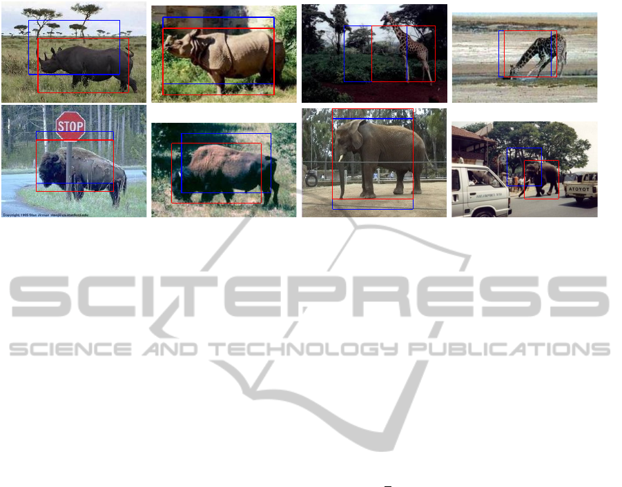
Figure 1: This figure shows, the final output of the object localization. In these examples, the training method was initialized
using the blue bounding boxes located at the center of the image. In the training framework, it is left to the training algorithm
to correctly converge to the location the objects with only the knowledge that this object has appeared in a number of images
and does appear in the others. As it can be seen in these examples, final output (red box) correctly points to the objects.
we formulate this problem as a weakly-supervised
clustering problem and show that the cluster centers
provide an efficient initialization for the Latent SVM
model (LSVM) (Felzenszwalb et al., 2010). To exper-
imentally evaluate our method, we look at the prob-
lem of object classification with latent localization.
This setup will provide us with an easy to evaluate
framework which is very challenging to solve. Fig. 1,
shows examples of this problem. In each image the
blue box is the location that is initially considered to
be the location of the object (In this case top left of
the image) and the red box is the location found after
the model is trained using the discussions in §3.
We organize this paper as following : In §2, we
provide a proper definition of the problem and discuss
strategies that can be used for initializing the latent
variable models. In §3, we propose an initialization
algorithm and in §4, we experimentally evaluate the
properties of this initialization and compare it with
other strategies. Finally, §5 concludes the paper.
2 PROBLEM DEFINITION
To formulate the problem, we assume that a dataset
of labeled images D = {(x
i
,y
i
)}
N
i=1
is provided with
x
i
being the image and y
i
∈ {−1,1} being the binary
label associated with it. For each image, there is a
latent variable h
i
∈ Z(x
i
) which localizes a fixed size
bounding box. The content of this bounding box is
encoded by the feature vector Φ(x
i
,h
i
) ∈ R
d
. In this
problem, the task of the learning algorithm is to clas-
sify the images x
i
according to the labeling y
i
while
correctly localizing the object. If the accurate value
of h
i
is known for the training examples then the
problem becomes a standard detector training prob-
lem. However, with the assumption that the value of
h
i
of the training images is undetermined, the training
task becomes significantly more challenging, because
for each image we do not know which value of h
i
points to the object and a wrong fixation of this value
can lead to training of inefficient models. The La-
tent SVM model (LSVM) (Felzenszwalb et al., 2010)
addresses this problem by minimizing the objective
function
L
D
(β) =
1
2
||β||
2
+C
N
∑
i=1
max(0,1 − y
i
f
β
(x
i
)), (1)
where
f
β
(x
i
) = max
z∈Z(x
i
)
β
T
Φ(x
i
,z). (2)
This optimization is usually done by iterating between
fixing the latent variables based on computed β and
optimizing the model parameters β over the fixed
problem. These iterations usually start by an initial
fixation of the latent variables. In this paper, we will
show that the outcome of this method is very sensi-
tive to the initialization and will discuss the effect of
different initializations on the solution.
When no prior knowledge of the object locations
is available, we can take several strategies to pick the
initial bounding box. In strategies such as picking the
center, top left or a random bounding box in the im-
age, the selection is done independent of the content
of the image. In these cases, the performance of the fi-
nal classifier depends on how good these initials over-
lap with the interest object. Unfortunately, guarantee-
ing this overlap without previous knowledge of the
object is not possible. To fix this, it is more desirable
for the initialization to be derived from the content
ICPRAM2014-InternationalConferenceonPatternRecognitionApplicationsandMethods
228

of the images. Since, we already know that the solu-
tion is an object that exists in within all the positive
images, it is natural to use a clustering procedure on
positive images to obtain a proper initialization. An
example of such a procedure, is to use the kmeans
algorithm to cluster the feature vectors coming from
the positive images. Each cluster center produces by
kmeans corresponds to certain feature vectors that re-
peats across the positive training samples. Using a
cross validation process it is possible to pick the most
representative center and use it to initially fix the la-
tent variables.
The problem with such a selection is the fact that
very few bounding boxes in each image actually cor-
respond to the object and these feature vectors will
most likely be ignored by a generic clustering algo-
rithm, due to lack of data. This brings the need for
an algorithm that can ignore the large and irrelevant
feature vectors and only focus on what is shared be-
tween the positive images. This is desired because a
feature vector that exists in all the positive images is
more likely to represent the object category. Such an
algorithm is presented in the following section.
3 LATENT OPTIMIZATION
To find feature vectors that are shared between the im-
ages, let D
+
contain only the positive images (|D
+
| =
M). For a given point p ∈ R
d
we define Ψ(x
i
, p) =
Φ(x
i
,z
?
i
(p)) where
z
?
i
(p) = argmin
z∈Z(x
i
)
kp − Φ(x
i
,z)k
2
. (3)
The aim of this section is to find a point p ∈ R
d
such
that the objective function
C
D
+
(p) =
1
M
∑
x
i
∈D
+
kp − Ψ(x
i
, p)k
2
, (4)
is minimized. In other words, we wish to find a fea-
ture vector that each positive image has a feature vec-
tor similar to it. To minimize this objective function,
we use an iterative method starting with a point p
(0)
(or equivalently an initial fixation of the latent vari-
ables) and calculate the next point as
p
(k+1)
=
1
M
∑
x
i
∈D
+
Ψ(x
i
, p
(k)
). (5)
Clearly, if for each x
i
, |Z(x
i
)| = 1 then this iteration
converges to the mean of the data after one step. How-
ever, because of the latent variables, the feature vec-
tor obtained from Ψ(x
i
, p
(k)
) changes with the change
of p
(k)
. This fact makes the behaviour this algorithm
more complex. The following theorem shows that this
iterative method minimizes the objective function 4.
Theorem 1. Given an imageset D
+
and p
(k)
and
p
(k+1)
defined as above, the following statement al-
ways holds :
C
D
+
(p
(k+1)
) ≤ C
D
+
(p
(k)
) (6)
Proof. To avoid clutter in the proof, for all p,q ∈ R
d
we define
∆
i
(p,q) = kp − Ψ(x
i
,q)k
2
. (7)
Since p
(k+1)
is calculated by Eq. 5, we can write
1
M
∑
x
i
∈D
+
∆
i
(p
(k+1)
, p
(k)
) ≤
1
M
∑
x
i
∈D
+
∆
i
(p
(k)
, p
(k)
).
(8)
This inequality assumes that the latent variables are
fixed by the point p
(k)
, and p
(k+1)
is simply the mean
of these fixed points. Due to the properties of mean,
the value of
1
M
∑
x
i
∈D
+
∆
i
( ˆp, p
(k)
) is the lowest when
ˆp = p
(k+1)
. We can also conclude from the definition
of Ψ(x
i
, p) that
∆
i
(p
(k+1)
, p
(k+1)
) ≤ ∆
i
(p
(k+1)
, p
(k)
). (9)
Combining the inequalities 8 and 9, gives us
C
D
+
(p
(k+1)
) ≤ C
D
+
(p
(k)
). (10)
This theorem shows that the iterative method dis-
cussed in this section will converge to a mode in R
d
with each points of this cluster coming from a differ-
ent image. Since this method only uses the positive
images, there is no guarantee that the found point ac-
tually corresponds to the object we are looking for.
To address this problem, Alg 1 sequentially finds k
distinct such points.
Fig. 2(Left), shows the behaviour of Alg. 1 on
synthetic data. In this data, each image is simulated
as a set of points randomly sampled from different
distributions (Explained in the appendix). This fig-
ure shows, how Alg. 1 converges to the data modes
and avoids already found distributions. In this exam-
ple, every set (image) contains at least one point from
each distribution. To highlight the difference between
kmeans and Alg. 1, we construct a slightly differ-
ent synthetic data. Here, rather than populating the
sets with points coming from all distributions, we di-
vide the sets in to two groups and follow a different
strategy for populating each group. As it can be see
in Fig. 2(Right), eight distributions are marked by
three colors {blue, cyan, magenta}. We sample from
blue and cyan distributions to construct the sets of the
first group and from magenta and cyan distributions
to construct the sets of the second group. Clearly,
the solution we are interested in should belong to all
InitializationFrameworkforLatentVariableModels
229

Algorithm 1: Finding shared representations.
Input: {(x
n
,L
x
n
)}
N
n=1
, k
Output: k cluster centers in the joint feature space
1: P ←
/
0 // Computed Centers
2: for i ← 1 to k do
3: p
(0)
i
← Randomly pick a vector from D
+
4: j ← 1
5: while not converged do
6: A
p
(i)
j
= {ψ(x,p
(i)
j
) : x ∈ D
+
}
7: A
(i)
j
← {a ∈ A
p
(i)
j
: ∀p ∈ P (ka − p
(i)
j
k < ka − pk)}
8: p
(i+1)
j
← (
∑
a∈A
(i)
j
a)/|A
(i)
j
|
9: j ← j + 1
10: end while
11: P ← P ∪ {p
?
j
}
12: end for
sets and come from a cyan distribution. We execute
kmeans on all the data points to find two cluster cen-
ters and execute Alg. 1 using the initial points demon-
strated in this figure. Here, it is expected from kmeans
to divide all the data points into two clusters. As it
can be seen, neither of the cluster centers found by
kmeans is close to the cyan distributions. On the other
hand, the centers found by 1, are located at the cen-
ter of both cyan distributions. In other words, while
kmeans tends to divide the data into several partitions,
Alg. 1 focuses on locating modes of the data with
the property that a feature vector close to them ex-
ists in every sample, a property that is not necessarily
true for the centers found by kmeans or other existing
clustering algorithms.
4 EXPERIMENTS AND RESULTS
To experimentally analyze the effects of the initial-
ization on the outcome of latent variable models, this
paper uses the mammals dataset (Heitz et al., 2009)
which has been used to benchmark the methods in
(Kumar et al., 2010; Yang et al., 2012) and follows
their experimental setting. In these experiments, it
is assumed that the objects have the same size and
the main challenge is considered to be the localiza-
tion of the object. To describe the image, we have
used the HOG descriptor (Dalal and Triggs, 2005;
Vedaldi and Fulkerson, 2008). The latent svm im-
plementation used in this paper is based on (Felzen-
szwalb et al., 2010) and as we can see in table 1, our
implementation slightly outperforms the results pre-
sented in (Yang et al., 2012) for linear models, using
the same assumptions. Each experiment is repeated
10 times on random splits of the dataset into training
and testing sets and the mean performance is reported.
Table 1: Comparison between the classification rates ob-
tained using different initialization methods. The large dif-
ference between these numbers shows the sensitivity of the
local variable models to initialization and how important it
to have robust methods for initializing them. In this table,
each experiment was repeated 10 times and the average per-
formance is reported. (*) Result from (Yang et al., 2012).
Init. Type Acc. %
Center 80.15 ± 2.79
Center (*) 75.07 ± 4.18
Random 66.93 ± 3.56
Top Left 61.75 ± 3.06
Kmeans (10 Centers) 69.85 ± 2.15
Alg. 1 (10 Points) 78.47 ± 3.91
As discussed in §2 and §3, we compare several
strategies of initialization {center, random, top left,
kmeans, Alg. 1 } and measure their effect as the per-
formance of the resulting detector on the test set.
• Center: In this case the initial location is selected
to be the center of each image. As we can see in
table 1, this initialization provides us with the best
performance despite the fact that this initialization
has nothing to do with the content of the image.
• Random: In this case the initial location is
selected randomly. Ideally on a non-biased
dataset the performance of the random initializa-
tion should be close to the center localization but
as we can see in table 1, there is a significant per-
formance drop when the random initialization is
used.
• Top Left: This initialization type was chosen to
make sure that initial locations has minimal over-
ICPRAM2014-InternationalConferenceonPatternRecognitionApplicationsandMethods
230

0 1 2 3 4 5 6 7
−1
0
1
2
3
4
Finding 4 cluster centers − Synthetic Data
All Points
k−means
Latent Opt m=15
Initial Point 1
Inital Point 2
Initial Point 3
Initial Point 4
0 1 2 3 4 5 6 7
0
1
2
3
4
5
6
Difference between Kmeans and Alg. 1 − Synthetic Data
Group A Points
Group B Points
Shared Points
Kmeans Centers
Alg. 1
Init. Points
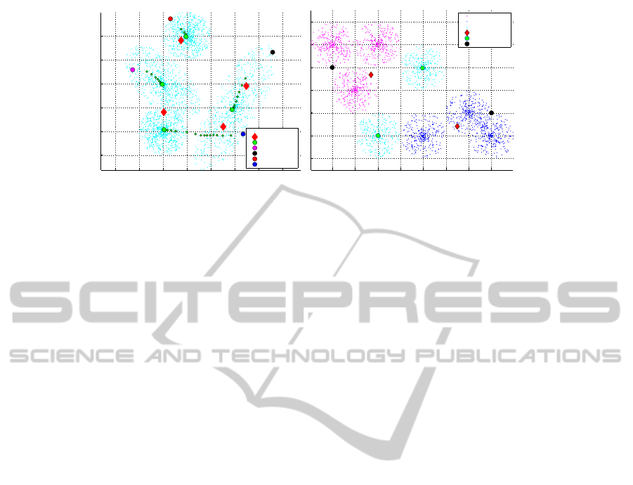
Figure 2: This figure shows the behaviour of Alg. 1 on synthetic data and compares it with the kmeans algorithm. As we
can see Alg. 1 converges to the center of the distributions and confirms our analysis in §3. (LEFT) To build the synthetic
data which simulates the conditions of the problem, 1500 data points were randomly sampled from 4 distributions. These
points were randomly distributed in 100 sets each containing 15 points. In this toy problem, each set was considered to be
a data sample with 15 different latent locations to choose from. (RIGHT) To show the difference between kmeans and Alg.
1, the synthetic data in this figure is produced by sampling from eight distributions are marked by three colors {blue, cyan,
magenta}. We have divided the sets into two groups with the first groups sampling from blue and cyan distributions and the
second sampling from magenta and cyan distributions. The distributions shared by all sets are the cyan distributions and as
we can see while the centers found by kmeans are not close to these distributions, Alg. 1 converges to the center of these
distributions.
lap with the target objects. As it can be seen in
table 1, the lowest performance is achieved when
this overlap is minimized.
• Kmeans: We use kmeans as a baseline for the per-
formance of Alg. 1. In order to use kmeans for
the initialization, we first cluster all the feature
vectors coming from the positive training set into
10 clusters. To pick which cluster center which
is the most representative, we divide the train-
ing set in half and cross validate LSVM method
while initialized with different centers. As it can
be seen in table 1, the performance significantly
improves compared to choosing a random initial-
ization. Here, once the most representative center
is selected, the LSVM is trained over the whole
training set and only this boundary is used for
evaluating the test images and no other informa-
tion is used at the testing stage.
• Alg. 1: Similar to the setting for kmeans, 10
modes were produced using Alg. 1 and the
most representative was used for initialization
of LSVM. Similarly, only the decision bound-
ary trained using the most representative center is
used at the testing stage. As it can be seen in table
1 the results significantly outperforms the base-
lines. A
It should be mentioned that in most cases there should
be no difference between the performance of center,
random, top left initialization strategies, due to the
fact that these initializations have nothing to do with
the content of the image. In the case of this problem,
the significant performance gained when the initial lo-
cation placed at the center of the image, comes from
the fact that most objects in this dataset are located in
the center and placing the initial location at the center
of the images gives the largest cover of the objects. In
other words, by doing so we assume that for most ob-
jects, we already know the location of the object. In
reality and on larger datasets, the performance of such
initialization should be closer to top left initialization
since the chance of covering the object using random
selection or picking the center location decreases.
5 CONCLUSIONS
In this paper, we have shown how different initializa-
tion strategies can effect the outcome of the LSVM
framework. To reduce the effects of the initialization,
we have formulated what a desired solution looks like
in terms of cluster centers and proposed an algorithm
for finding these cluster centers. As our experiments
show, LSVM framework trains a reasonably accu-
rate model using the initialization provided by our
method, without taking advantage of dataset bias or
being guided by user annotation.
ACKNOWLEDGEMENTS
This work was supported by The Swedish Foundation
for Strategic Research in the project Wearable Visual
Information Systems”.
InitializationFrameworkforLatentVariableModels
231

REFERENCES
Azizpour, H. and Laptev, I. (2012). Object Detection Us-
ing Strongly-Supervised Deformable Part Models. In
ECCV, pages 836–849.
Dalal, N. and Triggs, B. (2005). Histograms of Oriented
Gradients for Human Detection. In CVPR (1), pages
886–893.
Felzenszwalb, P. F., Girshick, R. B., McAllester, D., and
Ramanan, D. (2010). Object Detection with Dis-
criminatively Trained Part-Based Models. PAMI,
32(9):1627–1645.
Felzenszwalb, P. F. and Huttenlocher, D. P. (2005). Pictorial
Structures for Object Recognition. IJCV, 61(1):55–
79.
Heitz, G., Elidan, G., Packer, B., and Koller, D. (2009).
Shape-Based Object Localization for Descriptive
Classification. International Journal of Computer Vi-
sion, 84(1):40–62.
Kumar, M. P., Packer, B., and Koller, D. (2010). Self-Paced
Learning for Latent Variable Models. In Lafferty, J.,
Williams, C. K. I., Shawe-Taylor, J., Zemel, R. S., and
Culotta, A., editors, Advances in Neural Information
Processing Systems 23, pages 1189–1197.
Lowe, D. G. (2004). Distinctive Image Features from Scale-
Invariant Keypoints. International Journal of Com-
puter Vision, 60(2):91–110.
Vedaldi, A. and Fulkerson, B. (2008). VLFeat: An Open
and Portable Library of Computer Vision Algorithms.
Technical report.
Yang, W., Wang, Y., Vahdat, A., and Mori, G. (2012). Ker-
nel Latent SVM for Visual Recognition. In Bartlett,
P., Pereira, F. C. N., Burges, C. J. C., Bottou, L., and
Weinberger, K. Q., editors, Advances in Neural Infor-
mation Processing Systems 25, pages 818–826.
APPENDIX
SYNTHETIC DATA
Each image in the dataset D, can be see as a collec-
tion of different feature vectors. These feature vec-
tors usually come from many different distributions.
In the problem discussed in this paper, among all
these distributions we are interested in the distribu-
tions that each image in the dataset has a feature vec-
tor coming from that distribution. To build this data
synthetically, we assume that γ
1
,...,γ
n
are given dis-
tributions in R
d
and assume that each image is set
containing several points sampled from these distri-
butions. Each set is populated with m vectors where
each is obtained by randomly selecting a distribution
and sampling from it. This way each set simulates an
image with |Z(x)| = m. For d = 2, it is possible to
visualize the data points and get better understanding
of how the algorithms behave and visually compare
them with other algorithms.
ICPRAM2014-InternationalConferenceonPatternRecognitionApplicationsandMethods
232