Robot and Insect Navigation by Polarized Skylight
F. J. Smith and D. W. Stewart
School of Electronics, Electrical Engineering and Computer Science, Queens University Belfast, Belfast, N. Ireland
Keywords: Polarization, Skylight, Navigation, Clouds, POL, Robotic Navigation.
Abstract: A study of a large number of published experiments on the behaviour of insects navigating by skylight has
led to the design of a system for navigation in lightly clouded skies, suitable for a robot or drone. The
design is based on the measurement of the directions in the sky at which the polarization angle, i.e. the angle
χ between the polarized E-vector and the meridian, equals ±π/4 or ±(π/4 + π/3) or ±(π/4 - π/3). For any one
of these three options, at any given elevation, there are usually 4 such directions and these directions can
give the azimuth of the sun accurately in a few short steps, as an insect can do. A simulation shows that this
compass is accurate as well as simple and well suited for an insect or robot. A major advantage of this
design is that it is close to being invariant to variable cloud cover. Also if at least two of these 12 directions
are observed the solar azimuth can still be found by a robot, and possibly by an insect.
1 INTRODUCTION
That many insects can use the polarization in
skylight to navigate was first discovered in
experiments with bees by Karl von Frisch (1949).
The polarization of skylight had been already
discovered by the Irish Scientist Tyndall (1869) and
two years later a mathematical description of this
phenomenon was given by Lord Rayleigh (1871) for
the scattering by small particles (air molecules) in
the atmosphere, the basis of the theory in this paper.
Following von Frisch’s discovery it took another
25 years before the nature of the insect’s celestial
compass began to be clarified (
Kirschfeld et al., 1975;
Bernard and Wehner, 1977). It depends primarily
on a specialized part of the insect compound eye, a
comparatively small group of photoreceptors,
typically 100 in number, situated in the dorsal rim
area of each eye. Further insight on these
photoreceptors came from Wehner and co-workers
working with bees and desert ants (Labhart, 1980;
Rossel and Wehner, 1982; Fent and Wehner, 1985;
Wehner, 1997). It was found that each ommatidium
in the dorsal rim of the compound eye has two
photoreceptors, each strongly sensitive to the E-
vector orientation of plane polarized light, with axes
of polarization at right angles to one another. The
axes of polarization of the collection of these
ommatidia have a fan shaped orientation that has
been claimed from experiments to provide an
approximate map for the polarized sky, a map which
the insect can use as a compass (Rossel, 1993). The
variation in E-vector orientation has also been traced
within the central complex of the brain of an insect
(Heinze and Homberg, 2007).
Although much is known about this insect
compass little is known about the underlying
physical and mathematical processes that require
100 photoreceptors, the subject of this research.
One attempt has been made to design a navigational
aid for a robot based on the compass; this uses 3
pairs of photoreceptors (Wehner,1997; Lambrinos et
al, 1998), simulating the accumulation of results
from many photoreceptors in three different parts of
the fan of receptors used by an insect. This system
is reported to work well in the desert but there is no
evidence that this is mimicking the processes used
by insects; and it is not clear that this system would
be accurate under a variable cloudy sky. NASA has
also built robots navigating by skylight, but these
apparently use a different process based on 3
photoreceptors with 3 different axes of polarization
on a horizontal plane (NASA, 2005). Few details
have been released publicly on this system or its
performance.
It was proposed (Smith, 2008, 2009) that one fan
of photoreceptors is scanning the sky at a near
constant high elevation to find the 4 points in the sky
at this elevation, where the polarization angle, χ, the
angle between the meridian and the polarized E-
183
Smith F. and Stewart D..
Robot and Insect Navigation by Polarized Skylight.
DOI: 10.5220/0004792101830188
In Proceedings of the International Conference on Bio-inspired Systems and Signal Processing (BIOSIGNALS-2014), pages 183-188
ISBN: 978-989-758-011-6
Copyright
c
 2014 SCITEPRESS (Science and Technology Publications, Lda.)

vector, equals ±π/4. The anatomy of these
photoreceptors in bees, ants, and many other insects
is suitable to detect these four points.
In the first of these work-in-progress papers
(Smith, 2008) a simulation of this insect compass
was attempted using an algorithm involving 16
elements in a 4X4 array in which all possible solar
elevations were examined to find the correct one.
However, Wehner (1997) has shown that when
insects view the sky through two different windows
they obtain solar azimuths equal to the average of
the two azimuths obtained from each window. This
could not be explained as part of the above
algorithm. Nor was it compatible with a mapping of
the celestial compass in the insect brain by Heinz
and Homberg (2007).
These results led to the discovery of a simpler
algorithm (Smith, 2009) for this single fan of
photoreceptors. However, many insects have
ommatidia in sets of three fans with the polarization
axes of the 3 sets differing by about π/3 (Labhart,
1988; Wehner, 2001). This has led to the expansion
of the algorithm in this paper.
Also, the invariance to cloud cover was not fully
understood. We show here that this invariance is
linked to the fields of view of the observations.
2 THEORY
When partially polarized skylight enters an
ommatidium in the dorsal rim its intensity is
measured by two photoreceptors, each of which can
measure polarized light with parallel structures
called microvilli. The two directions of the
microvilli are at right angles to one another, and
define two orthogonal axes of polarization for these
X and Y photoreceptors. The orientations of the
microvilli in the dorsal rim of the honey bee were
found to vary continually from the front to the back
of the head in a fan shape (Sommer, 1979), the X
photoreceptor measuring light polarised roughly
parallel to the meridian on the other side of the head
(Rossel, 1993). The same approximate parallel
pattern was found in desert ants by Wehner and
Raber (1979), and later in several other insects. Two
other similar fans of photoreceptors were also
discovered in many insects with microvilli
orientated at +π/3 and -π/3 with the first.
In a simulation of skylight based on Rayleigh’s
theory (1871) expressions were derived (Smith,
2008) for the light intensities, S
X
and S
Y
, measured
by the two receptors, named X and Y. If U is the
intensity of unpolarized light (due to multiple
scattering), if θ is the scattering angle of the light
scattered once only at the centre of the patch of sky
being observed and if ξ is the angle which the
microvilli (S
X
) make with the meridian then:


UPS
X
 )(sin)(sin1
22

(1)


UPS
Y
 )(cos)(sin1
22

(2)
where the factor P depends on terms derived by
Rayleigh (1871) and on the measuring capability of
the photoreceptors.
It has been shown by Labhart (1988) that the
brain of a cricket records the difference between the
two signals, S
Y
and S
X
is the form:
)()(
XYYX
SLogSLogS


(3)
We illustrate the variation in these signals as the
observation azimuth angles, a
o
, of the ommatidia
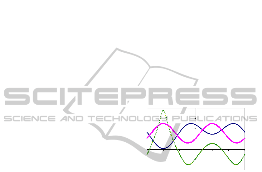
vary in Figure (1) due to a point source.
Figure 1: Illustration of the signals S
X
S
Y
and S
YX
in a blue
sky [U=0] as they vary with the azimuth, a
o
, of the fan of
observations measured from the central axis of the insect
with ξ=0, with solar elevation h
s
=30
o
, and solar azimuth
a
s
=60
o
. Note that there are 2 maxima and also 4 azimuths
Z where S
X
=S
Y
or S
YX
=0, called zeros.
3 INVARIANCE TO CLOUD
We need to know first why insects are measuring the
difference S
YX
between the signals from the two
orthogonally polarized photoreceptors rather than S
Y
.
Is it eliminating the greatest problem, variable cloud
represented by U? Certainly S
YX
reduces the effect
of U, but it does not remove it. This is illustrated in
Figure 2 where clouds are simulated for the example
in Figure 1.
3.1 Maxima, Minima, Zeros
It appears from Figure 2 that little information can
be obtained from the absolute values of S
YX
. But the
‐0.8
‐0.4
0
0.4
0.8
1.2
1.6
‐180 ‐120 ‐60
0
60 120 180
ao
o
BlueSky
Syx
Sy
Sx
BIOSIGNALS2014-InternationalConferenceonBio-inspiredSystemsandSignalProcessing
184

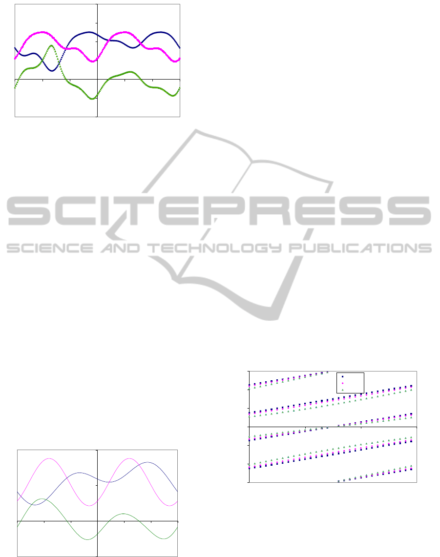
Figure 2: Example in Figure 1 with simulated cloud added
[U=0.5 sin
2
(a
o
), P=1-U].
positions of the maxima vary little from Figure (1)
and are largely invariant to the cloud. These
maxima occur in the directions of the solar meridian,
a
s
, and of the antisolar meridian, a
s
+π. In both these
directions S
Y
goes through a maximum while S
X
goes
through a minimum. So the difference goes through
an enhanced maximum (Labhart, 1988). Either of
these maxima can give the direction of the sun.
The two minima cannot be used reliably because
the minima of S
Y
do not coincide with the maxima in
S
X
: they may be as much as 20
o
different, because
sin
2
(θ) in Equations (1) and (2) is not stationary as it
is at the maxima.
A close examination of Figures (1) and (2) shows
that the positions of the 4 zeros in S
YX
have not
changed. This invariance can be proved
mathematically from Equations 1 & 2 for a point
source. However, a point source, that is a narrow
window of observation, is not practical if an insect
or robot is to measure the sometimes small
difference between the signals S
X
and S
Y
. So each
ommatidium observes the sky with a wide angle of
observation. The affect of such a wide angle on the
cloud cover is illustrated in Figure 3 for the same
example as in Figure 2.
Figure 3: The intensities in Figure 2 viewed through a
wide window: h
o
from 45
o
to 90
o
, a
o
from 80
o
to 90
o
.
Figure 3 shows that a wide field of view does
smooth out the impact of small variable cloud, but it
does not eliminate it. The positions of the maxima
in S
xy
are still changed, but less than before, but now
a close examination shows that the positions of the
zeros have changed also. So the necessary wider
angle of observation can introduce a small error in
the position of the zeros.
Fortunately observations in real cloudy skies
have been published with 2 wide windows by
Labhart (1999). An analysis of these data shows
that the errors caused by cloud in the positions of the
maxima were small, mostly 3
o
or less. The errors in
the zeros were lower, mostly 1.5
o
or less, but they
are lower still when the window of observation is
smaller, supporting the above results.
3.2 4 Zeros
So the possibility is that S
YX
is measuring the
positions of the 4 zeros. Mathematically, putting S
YX
= 0 or S
X
=S
Y
in Equations (1 to 3) brings about a
large simplification eliminating the unknowns U, P
and θ in one step and reducing the equations to:
sin
2
(χ-ξ) = cos
2
(χ-ξ). This makes χ-ξ = ±π/4. So
finding the zeros where S
YX
=0 gives us the azimuths
Z where χ = ξ±π/4. Examples of zeros for different
solar elevations and values of ξ for a constant
elevation of observation h
o
=80
o
are shown in Figure
(4). There are always 4 zeros for each ξ if the
window of observation is at a constant elevation.
However, when the solar elevation is above the
observation elevation there may be no zeros.
Figure 4: Azimuths a
o
of the 4 zeros relative to the sun
(a
s
=0) of zeros where S
YX
= 0 and χ=ξ±π/4 plotted against
the angle ξ for 3 elevations of the sun el = 0
o
, 30
o
and 60
o
.
To calculate the positions of the zeros we need
the polarization angle, χ, in terms of the solar
azimuth, a
s
and the solar elevation, h
s
along with the
azimuth, a
o
, and elevation, h
o
, of the centre of the
patch of sky being observed by the photoreceptor.
In a previous paper (Smith, 2008) it was shown
-0.8
-0.4
0
0.4
0.8
1.2
1.6
-180 -120 -60 0 60 120 180
Syx
Sy
Sx
Clouded Sky
ao
-0.8
0
0.8
1.6
-180 -120 -60 0 60 120 180
Sy
Sx
Syx
ao
-180
-120
-60
0
60
120
180
0306090
el=0
el=30
el=60
ξ
ao
RobotandInsectNavigationbyPolarizedSkylight
185

using geometry and vector algebra and noting that if
ξ = 0 then cos(χ) = 1 and sin(χ) = ±1 at the zeros; so
)tan()cos()sin()sin()cos(
soo
hhaha 
(4)
where a = a
s
– a
o
is the azimuth of the sun relative
to the azimuth of the observed sky. Solving this for
a
s
, the azimuth of the sun, gives expressions for a
s
,
for the 4 zeros, Z
i
, i = 1..4:




is
Za
(5)
in which δ = arccos(tan(h
s
)cos(h
o
)/K) and γ =
arcsin(1/K) where K
2
= 1+ sin
2
(h
o
). If the sky is
scanned at a constant elevation h
o
then the angles γ
and δ are constant. (If ξ ≠ 0 both γ and δ change
because K
2
= tan
2
(ξ ± π/4)+ sin
2
(h
o
)). The angle γ
depends only on the elevation of the observation,
determined by the geometry of the ommatidium of
the insect or robot and is therefore known; it is large,
>π/4. The angle δ depends on the solar elevation and
when the sun is on the horizon it equals π/2 (since
tan(h
s
)=0). It can be calculated by a robot from the
above equation for δ, which needs the solar
elevation, known from the latitude and time.
Fortunately we now show that this difficult
calculation is not needed by an insect.
4 THE ALGORITHMS
4.1 Ommatidia with ξ =0
We begin with the fan of observations when ξ=0
because, as evident from Figures 4 and 5, this is the
only value of ξ for which there is symmetry on either
side of the solar azimuth. The 4 alternatives in
Equation (5) correspond to the four zeros as
illustrated in Figure (5), which we write as
a
s
= Z
1
+ γ – δ, a
s
= Z
2
– γ – δ
(6)
a
s
= Z
3
– γ + δ, a
s
= Z
4
+ γ+ δ (7)
where the signs are chosen by symmetry in the
geometry in Figure (5). Note that all of these
quantities are large angles in [0,2π]; so the sums are
all modulus 2π.
If we sum these 4 expressions, the γ and δ terms
cancel and we get 4a
s
= Z
1
+Z
2
+Z
3
+Z
4
, mod 2π.
Dividing by 4 gives a
s
, but because of the cyclic
nature of the summation (350
o
+ 20
o
= 10
o
) an
uncertainty of mπ/2 occurs where m=0, 1, 2 or 3.
This uncertainty can be resolved by noting in Figure
5 that (1) Z
2
– Z
1
= Z
4
– Z
3
and (2) the two zeros Z
1
and Z
4
nearest to the sun are closer together than the
other two. These two conditions are used in the
following algorithm to calculate a
s
from 4 measured
zeros, Y
1
, Y
2
, Y
3
, and Y
4
, where at first the order is
not known, i.e. which one of them is Z
1
in Figure 5.
Figure 5: Example of the approximate directions of the 12
zeros where S
YX
= 0 relative to the direction of the sun for
a solar elevation h
s
= 60
o
, 4 zeros marked Z1, Z2, Z3 and
Z4 for ξ =0 (black), 4 zeros for ξ = +60
o
(green) and 4
zeros for ξ = -60
o
(red).
So the algorithm (for ξ =0) is:
1. find the 4 zeros in [0, 2π] where S
X
= S
Y
;
2. put in order Y
1
, Y
2
, Y
3
, and Y
4
;
3. find the sum: S = Y
1
+ Y
2
,+ Y
3
+ Y
4
;
4. put i=1; m=0;
5. if y
2
– y
1
<> y
4
– y
3
then i=2 and m=1;
6. if y
i
– y
i+3
< y
i+2
– y
i+1
then m=m+2;
7. a
s
= (S/4 + m*π/2) mod 2π.
(Note that differences are cyclical and clockwise.)
For example, for a solar elevation h
s
= 60
o
and
observation elevation h
o
= 80
o
assume that we find 4
zeros at azimuths: 70
o
, 134
o
, 225
o
, and 339
o
.
Following the algorithm we find that m=3 and Y
4
=
Z
1
, S=768
o
, S/4=192
o
and a
s
=192
o
+270
o
=462
o
=102
o
,
the correct solar azimuth. Simulations with about
5000 examples for ξ = 0 have shown that this
algorithm succeeds in almost every case with no
ambiguity within a tolerance of 1 degree. Errors
occur only at very low or high solar elevations ( ≤ 2
o
or > h
o
).
4.2 Less than 4 Zeros Observable
Sometimes not all of the 4 zeros for ξ = 0 are
observable. If only one zero can be observed
because much of the sky is obscured then we have 4
possible values for the direction of the sun, a
s,
given
by Equations (6) and (7) and it is not known which
is correct without more information (such as a light
intensity maximum in one of the 4 directions).
If 2 or 3 zeros with ξ = 0 can be found an insect
Z1
Z2Z3
Z4
BIOSIGNALS2014-InternationalConferenceonBio-inspiredSystemsandSignalProcessing
186

appears to use the average of the detectable zeros
(Wehner, 1997). The angle γ is a known constant for
the ommatidium but the angle δ is probably too
difficult to calculate for an insect (see Section 3.2);
so it puts δ = π/2, assuming that the sun is on the
horizon (Rossel & Wehner, 1982), and uses the
average of the available values: z ± γ ± π/2. This
leaves an error of ±(δ-π/2) if one zero only is
observed; but if 2 zeros are observed then the
average of the two zeros gives either the same error
±(δ-π/2) or, if they are symmetric about the solar
meridian, an error of zero.
The errors obtained from the above equations are
in general agreement with experimental data with
insects by Wehner (1989). This supports the
proposal that the insect compass is based primarily
on the 4 zeros if ξ = 0.
4.3 Ommatidia with ξ = ± π/3
However, we know that some insects, at least, also
have ommatidia with ξ = +π/3 and –π/3. It is not
likely that they are doing this to find the position of
the maxima in the S
XY
signal, but more likely to
increase the number of zeros they can observe in a
cloudy sky. If ξ ≠ 0 then the symmetry used in the
algorithm in Section 4.1 is lost as evident from
Figure (5). However, an examination of Figure 5
also shows that there is reverse symmetry between
the 4 zeros for ξ = +60
o
and for ξ = -60
o
. For the
example in Figure 5 the 4 zeros for ξ = +60
o
are
clockwise
+69
o
, +164
o
, -100
o
and -13
o
.
and the zeros for ξ= -60
o
are
+13
o
, +100
o
, -164
o
and -69
o
.
So the algorithm in Section 4.1 can be used with the
average of the first two zeros in one set with the last
two in the second set to find the solar azimuth.
Although there are other possibilities, for
example, the average of the 12 zeros for ξ = 0 and
±60
o
together might be used for a blue sky, it is more
likely that the real value of the extra zeros is when a
few of the 4 zeros for ξ = 0 are not available. It is
similar for a robot.
5 ROBOT DESIGN
There are two parts to the robot design: (1) the
optics for the measurement of the zeros and (2) the
algorithms to calculate a
s
. This paper is primarily
concerned with the algorithms and we discuss the
geometry of the optics only briefly.
The robot optics can generally follow the insect
design with fans of pairs of orthogonally orientated
micro photo-detectors scanning the sky at a constant
high elevation. This is not easy; so alternatively a
single highly sensitive rotating detector might do the
same task. Like an insect it would use 3 fans of
photoreceptors. (To avoid ξ=π/4 which has only 2
zeros, sets of 2 or 4 fans could not be used, and 5 or
more would involve redundancy.) The field of view
would be kept small to keep errors due to clouds at a
minimum; but there is a trade-off between errors and
sensitivity to light in the robot, as there is in an
insect. Unlike an insect it would help if each
photoreceptor could use one lens with 3 pairs of
orthogonally orientated sensors, so that they can all
view the same patch of sky together. But like most
insects the system would detect ultraviolet light
which can penetrate cloud more easily than visible
light (Pomozi et al., 2001).
The Robot algorithm has one advantage over an
insect that it can compute the δ terms in Equations
(6) and (7) accurately. This corrects the error that
some insects make by always putting δ = π/2 (see
Section 4.2). Since the γ term is also known this
permits a different algorithm by a robot when at
least 2 zeros, Z
1
and Z
2
not necessarily with the same
ξ, are known out of the 12. Since the γ and δ terms
in equations (6) and (7) may not be the same we
rewrite them as
a
s
= Z
1
± γ
1
± δ
1
(8)
a
s
= Z
2
± γ
2
± δ
2
(9)
where δ
1
and γ
1
correspond to Z
1
and δ
2
and γ
2
correspond to Z
2
. There are four possibilities in each
equation with only one correct, but the correct one
gives the same a
s
in both cases. So an alternative
algorithm scans through the 4 X 4 = 16
combinations of Equation (8) with Equation (9) to
find the closest match. The average of the two then
gives a
s
. If γ
1
= γ
2
= γ and δ
1
= δ
2
= δ then the
algorithm is unchanged but there are fewer
alternatives.
If a third zero is found then this process is
repeated and an average of the three is taken. The
same process continues for each additional zero
observed up to 12 giving increasingly more accurate
values for a
s
. It is possible that an insect does
something similar with all δ’s replaced by π/2.
RobotandInsectNavigationbyPolarizedSkylight
187

6 CONCLUSIONS
We have shown that an accurate celestial compass
for an insect or robot can be built round the principle
of finding in skylight at a constant elevation the 12
azimuths at which χ = ± π/4 or ± π/4 ± π/3, called
zeros. One algorithm described for this compass is
simple and accurate and well within the capacity of
an insect to navigate continuously. It also explains
many experiments on insect behaviour. A closely
related algorithm is more appropriate for a robot,
relying on its greater computational ability to correct
an error sometimes made by insects.
Besides the simplicity and accuracy of the
method its greatest advantage is that it is accurate in
hazy and partially clouded skies, because the
positions of the zeros are almost unchanged by cloud
particularly if the window of observation is not too
large.
For the method to be accurate the top of the robot
or drone must be pointing accurately towards the
zenith. Insects may do this using 3 separate ocelli
on the top of their heads (Goodman, 1970). But how
they do this is not yet known. This needs more
experimental evidence on the anatomy and
behaviour of insects.
More experiment is vital to test that the
theoretical simulations and conjectures in this paper
are correct or otherwise with a working robotic
system. Tests on the behaviour of insects viewing
the zeros for ξ = +π/3 or –π/3 are also needed and
are planned.
REFERENCES
Bernard, G. D., Wehner, R., 1977. Functional similarities
between polarization vision and color vision, Vision
Res., 17, 1019-28.
Fent, K., Wehner, R, 1985. Ocelli: A celestial compass in
the desert ant Cataglyphis, Science, 228, 192-4.
Goodman, L. J., 1970. The structure and function of the
insect dorsal ocellus. Adv. Insect Phys., 7, 97-195.
Heinze, S., Homberg, U., 2007. Maplike Representation of
Celestial E-Vector Orientations in the Brain of an
Insect, Science, 315, 995-7.
Kirschfeld, K., Lindauer, M., Martin, H., 1975. Problems
in menotactic orientation according to the polarized
light of the sky, Z. Naturforsch, 30C, 88-90.
Labhart, T., 1980. Specialized Photoreceptors at the dorsal
rim of the honeybee’s compound eye: Polarizational
and Angular Sensitivity, J Comp. Phys., 141, 19-30.
Labhart, T., 1988. Polarized-opponent interneurons in the
insect visual system, Nature, 331, 435-7.
Labhart, T., 1999. How polarization-sensitive
interneurones of crickets see the polarization pattern of
the sky: a field study with an optoelectronic model
neurone, J. Exp. Biol., 202, 757-70.
Lambrinos, D., Maris, M., Kobayashi, H., Labhart, T.,
Pfeifer, P., Wehner, R., 1998. Navigation with a
polarized light compass, Self-Learning Robots II: Bio-
Robotics (Digest 1998/248) IEE, London, 7/1-4.
NASA,2005. www.nasatech.com/Briefs/Oct05/
NPO_41269.html.
Pomozi, I., Horvath, G., Wehner, R., 2001. How the
clear-sky angle of polarization pattern continues
underneath clouds, J. Expt. Biol, 204, 2933-42.
Rayleigh, Lord, 1871. On the light from the sky, its
polarisation and colour, Phil Mag, 41, 107-20, 274-9.
Rossel, S., 1993. Mini Review: Navigation by bees using
polarized skylight, Comp. Biochem. Physiol, 104A,
695-705.
Rossel, S., and Wehner, R., 1982. The bee’s map of the e-
vector pattern in the sky, Proc. Natl. Acad. Sci. USA,
79, 4451-5.
Sommer, E. W., 1979. Untersuchungen zur topo-
graphischen Anatomie der Retina und zur
Sehfeldoptologie im Auge der Honigbiene, Apis
mellifera (Hymenoptera). PhD Thesis, Un. Zurich.
Smith, F. J., 2008. A new algorithm for navigation by
skylight based on insect vision, in Biosignals 2008, 2,
Eds. P Encarnacao & A Veloso, Madeira, 185-90.
Smith, F. J., 2009. Insect Navigation by Polarised Light in
Biosignals 2009, 2, Porto, Portugal, 363-8.
Tyndall, J., 1869. On the blue colour of the sky, the
polarisation of skylight, and on the polarisation of
cloudy matter, Proc. Roy. Soc., 17, 223.
Von Frisch, K., 1949. Die Polarization des Himmelslichts
als Orientierender Faktor bei den Tanzen der Bienen,
Experientia, 5, 142-8.
Wehner, R., 1989. The hymenopteran skylight compass:
matched filtering and parallel coding, J Exp. Biol.
,
146, 63-85.
Wehner, R., 1997. The Ant’s celestial compass system:
spectral and polarization channels, In Orientation and
Communication in Arthropods, Ed. M. Lehler,
Birkhauser, Berlag, Basel, Switzerland, 145-85.
Wehner, R., and Raber, F., 1979. Visual spatial memory in
desert ants, Cataglyphis bicolor (Hymenoptera:
Formicidae), Experientia, 35, 1569-71.
Wehner, R., 2001. Polarization vision – a uniform sensory
capacity, J. Exp. Biol., 204, 2589-96.
BIOSIGNALS2014-InternationalConferenceonBio-inspiredSystemsandSignalProcessing
188