
Learning on Vertically Partitioned Data based on Chi-square Feature
Selection and Naive Bayes Classification
Ver´onica Bol´on-Canedo, Diego Peteiro-Barral, Amparo Alonso-Betanzos, Bertha Guijarro-Berdi˜nas
and Noelia S´anchez-Maro˜no
Department of Computer Science, University of A Coru˜na, Campus de Elvi˜na s/n, A Coru˜na 15071, Spain
Keywords:
Feature Selection, Classification, Distributed Learning.
Abstract:
In the last few years, distributed learning has been the focus of much attention due to the explosion of big
databases, in some cases distributed across different nodes. However, the great majority of current selection
and classification algorithms are designed for centralized learning, i.e. they use the whole dataset at once. In
this paper, a new approach for learning on vertically partitioned data is presented, which covers both feature
selection and classification. The approach splits the data by features, and then uses the χ
2
filter and the
naive Bayes classifier to learn at each node. Finally, a merging procedure is performed, which updates the
learned model in an incremental fashion. The experimental results on five representative datasets show that the
execution time is shortened considerably whereas the classification performance is maintained as the number
of nodes increases.
1 INTRODUCTION
In the last decades, the dimensionality of the datasets
involved in data mining has increased dramatically
until the size of zetabytes. In fact, if one analyzes the
dimensionality of the datasets posted in the UC Irvine
Machine Learning Repository (Frank and Asuncion,
2010) from 1987 to 2010, this circumstance can be
confirmed (Zhao and Liu, 2011). Dimensionality can
be defined as the product of the number of samples
and features. In the 1980s, the maximal dimensional-
ity of the data was about 100; then in the 1990s, this
number increased to more than 1500; and finally in
the 2000s, it further increased to about 3 million. The-
oretically, having such a high amount of data avail-
able could lead to better results, but this is not always
the case due to the so-called curse of dimensional-
ity (Bellman, 1966). This phenomenon happens when
the dimensionality increases and the time required for
training the machine learning algorithm on the data
increases exponentially. To overcome these problems,
feature selection is a well-known dimensionality re-
duction technique.
Feature selection consists of detecting the relevant
features and discarding the irrelevant and the redun-
dant ones (Guyon et al., 2006). A correct selection of
the features can lead to an improvement of the induc-
tive learner, either in terms of learning speed, gener-
alization capacity or simplicity of the induced model.
Feature selection, since it is an important activity in
data preprocessing, has been an active research area
in the last decade, finding success in many different
real world applications (Bol´on-Canedo et al., 2011;
Forman, 2003; Saari et al., 2011; Saeys et al., 2007).
Most of the feature selection methods belong to
one of the three following types: filters, wrappers and
embedded methods. While wrapper models involve
optimizing a predictor as part of the selection process,
filter models rely on the general characteristics of the
training data to select features with independence of
any predictor. The embedded methods generally use
machine learning models for classification, and then
an optimal subset of features is built by the classi-
fier algorithm. Nevertheless, the most common ap-
proach in feature selection is the filter model and will
be the approach selected for this research, As stated
in (Saeys et al., 2007), even when the subset of fea-
tures is not optimal, filters are preferable due to their
computational and statistical scalability.
Most existing feature selection techniques are de-
signed to run in a centralized computing environ-
ment. Traditionally, it is assumed that all data can
be held in the memory or, at least, all data are stored
in one central storage space. However, in the con-
temporary world, huge databases are developed and
maintained in meteorological, financial, medical, in-
350
Bolón-Canedo V., Peteiro-Barral D., Alonso-Betanzos A., Guijarro-Berdiñas B. and Sánchez-Maroño N..
Learning on Vertically Partitioned Data based on Chi-square Feature Selection and Naive Bayes Classification.
DOI: 10.5220/0004759503500357
In Proceedings of the 6th International Conference on Agents and Artificial Intelligence (ICAART-2014), pages 350-357
ISBN: 978-989-758-015-4
Copyright
c
2014 SCITEPRESS (Science and Technology Publications, Lda.)

dustrial or science domains (Czarnowski, 2011), and
traditional centralized techniques are not fit to effec-
tively deal with such massive datasets. Not only is the
large size of the datasets the problem facing feature
selection, but also that the datasets may be geographi-
cally, physically or logically distributed. In both these
situations, distributed feature selection techniques are
often required. In this manner, allocating the learn-
ing process among several nodes is a natural way of
scaling up learning algorithms at the same time that
it allows to deal with datasets that are naturally dis-
tributed. There are two common types of data distri-
bution: (a) horizontal distribution, where data are dis-
tributed in subsets of instances; and (b) vertical dis-
tribution, where data are distributed in subsets of fea-
tures. The great majority of approaches distribute the
data horizontally (Chan et al., 1993; Ananthanarayana
et al., 2000; Tsoumakas and Vlahavas, 2002) when
datasets are too large for batch learning in terms of
samples. While not common, there are some other de-
velopments that distribute the data by features (Skil-
licorn and McConnell, 2008; McConnell and Skil-
licorn, 2004), which is appropriate when the number
of features is large. Besides of the type of partition,
another important issue when dealing with distributed
learning is privacy preserving. The goal of privacy
preserving is to learn valuable knowledge from dif-
ferent sources without leakage of any sensitive data,
in other words, share non-sensitive data to infer sen-
sitive data (Wang et al., 2009).
The idea of this research is to deal with distributed
learning problems through distributing vertically the
data and performing a feature selection process which
can be carried out at separate nodes. Since the compu-
tational complexity of most of feature selection meth-
ods is affected by the number of features, the com-
plexity in each node will be reduced with respect to
the centralized approach. Then, the selection pro-
cedure required for the data reduction will be inte-
grated with the classifier learning. For the feature se-
lection step, we choose the χ
2
metric (Liu and Se-
tiono, 1995), because of its simplicity and effective-
ness. However, this filter requires data to be discrete,
so a discretization stage has to be added to prepro-
cess the data. Finally, a classifier is necessary, and
the well-known naive Bayes (Rish, 2001) was cho-
sen. This decision has been made because after per-
forming the three stages in each node (discretization,
selection and classification), the learned models are
combined in a incremental manner, and naive Bayes
has some characteristics that makes it inherently in-
cremental. With the proposed methodology, it is ex-
pected that the global learning process will be sped up
and so become more computationally efficient.
The rest of the paper is organized as follows: sec-
tion 2 presents the state of the art in the field of dis-
tributed learning, section 3 describes the method pro-
posed in this research, section 4 introduces the ex-
perimental settings and results and, finally, section 5
reveals the conclusions and future lines of research.
2 BACKGROUND AND RELATED
WORK
Most of the research in the literature concerning dis-
tributed learning proposes privacy-preserving meth-
ods for horizontally partitioned data. A meta-learning
approach has been developed that uses classifiers
trained at different sites to develop a global classi-
fier (Prodromidis et al., 2000). In (Wolpert, 1992;
Chawla et al., 2002; Tsoumakas and Vlahavas, 2002;
Kantarcioglu and Clifton, 2004; Tsoumakas and Vla-
havas, 2009), the authors proposed several privacy-
preserving classification methods for horizontally
partitioned data. However, previous research in dis-
tributed classification for vertically partitioned data is
rather sparse. In (Vaidya and Clifton, 2005), it is in-
troduced a generalized privacy preserving variant of
the ID3 algorithm for vertically partitioned data dis-
tributed over two or more parties. In (Vaidya and
Clifton, 2004), the authors addressed classification
over vertically partitioned data where either all the
parties hold the class attribute, or only a subset of
the parties have the class attribute. The basic idea
behind their protocol is that each party ends up with
shares of the conditionally independent probabilities
that constitute the parameters of a Na¨ıve Bayes clas-
sifier. In (Gangrade and Patel, 2013), all party cal-
culates probabilities (model parameters of a Na¨ıve
Bayes classifier) of all class value for each attribute
value for every attribute individually, causing no pri-
vacy breaches. They use secure multiplication pro-
tocol for multiplying the probabilities of particular
values of all attributes for all class value and com-
pare total probability of all class value and find out
the maximum total probability. Other research has
addressed classification using Bayesian networks in
vertically partitioned data (Chen et al., 2001), and sit-
uations where the distribution is itself interesting with
respect to what is learned (Wirth et al., 2001).
On the other hand, regarding distributed feature
selection, a distributed privacy-preserving method to
perform feature subset selection that handles both
horizontal as well as vertical data partitioning is pro-
posed in (Banerjee and Chakravarty, 2011). In that
paper a secure distributed protocol was proposed.
It allows feature selection for multiple parties with-
LearningonVerticallyPartitionedDatabasedonChi-squareFeatureSelectionandNaiveBayesClassification
351
out revealing their own data evolving from a method
called virtual dimension reduction. This method is
used in the field of hyperspectral image process-
ing for selection of subset of hyperspectral bands
for further analysis. In (Ye et al., 2010), the au-
thors addressed attribute reduction over vertically par-
titioned data, where two parties, each having a pri-
vate dataset want to collaboratively conduct global at-
tribute reduction. By using a semi-trusted third party
and commutative encryption, they presented some se-
cure multi-party computation (SMC) protocols (Yao,
1982) into privacy preserving attribute reduction al-
gorithms. But the method is only proven secure under
the semi-honest model, and security under this ad-
versary model is insufficient. SMC protocols under
the malicious adversary model generally have imprac-
tically high complexities for privacy-preserving data
mining.
As can be seen, distributed classification algo-
rithms are becoming more popular in machine learn-
ing. Moreover, some first steps are taken towards de-
veloping distributed feature selection methods. How-
ever, to the best knowledge of the authors, none of the
previous research addresses both distributed feature
selection and classification simultaneously on verti-
cally partitioned data.
3 THE PROPOSED METHOD
As stated before, distributed feature selection on ver-
tically partitioned data has not been deeply explored
yet. Distributed methods usually consist of three
stages:
1. Partition of the dataset (if the dataset is not dis-
tributed from origin).
2. Application of learning methods in each node. In
the case of the method proposed herein, it consists
of three steps:
(a) Discretization.
(b) Feature selection.
(c) Classification.
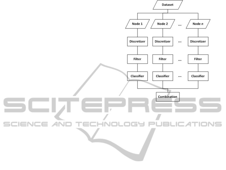
3. Combination of the results.
The interest of this work relies on the independence
of the methodology, that can be performed on all the
nodes at the same time. Besides, the novelty in the
combination stage is that it is done in an incremental
manner. As explained before, the learning methodol-
ogy to be applied to each node consists of three steps:
discretization, feature selection and classification (see
Figure 1).
Figure 1: Flow chart of proposed methodology.
3.1 Partition of the Dataset
In some cases, data can be originally distributed by
features. In this manner, different features belonging
to the same sample are recorded in different locations.
Each node gathers the values for one or more features
for a given instance and then, each node has a differ-
ent “view” of the data. For instance, a sensor network
usually records a single feature in each sensor. An-
other example may be a patient that performs several
medical tests in different hospitals. In such these sit-
uations, a distributed learning approach can be much
more efficient computationally than moving all dis-
tributed datasets into a centralized site for learning the
global model. Moreover,even when data are stored in
a single site, distributed learning can be also useful to
speed up the process.
As most of the datasets publicly available are
stored in a centralized manner, the first step consists
of partitioning the dataset, i.e. dividing the original
dataset into several disjoint subsets of approximately
the same size that coverthe full dataset. As mentioned
in the introduction, in this research the partition will
be done vertically, as can be seen in Figure 2. Notice
that this step could be eliminated in a real distributed
situation.
3.2 Learning Methods
In this research, the learning stage consists of three
steps: discretizer, filter and classifier, which will be
following described.
ICAART2014-InternationalConferenceonAgentsandArtificialIntelligence
352

Figure 2: Vertical partition of the data.
3.2.1 Discretizer
Many filter algorithms are shown to work effectively
on discrete data (Liu and Setiono, 1997), so dis-
cretization is a recommended as a previous step. The
well-known k-means discretization algorithm (Tou
and Gonz´alez, 1977; Ventura and Martinez, 1995)
was chosen because of its simplicity and effective-
ness. K-means moves the representative weights of
each cluster along an unrestrained input space, where
each feature is discretized independently, making it
suitable for our purposes. This clustering algorithm
operates on a set of data points and assumes that
the number of clusters to be determined (k) is given.
The partition is done based on certain objective func-
tion. The most frequently used criterion function in k-
means is minimizing the squared error ε between the
centroids µ
i
of clusters c
i
,i = 1,... ,k and the samples
in those clusters
ε =
∑
x∈c
i
|x− µ
i
|
2
Let C be the set of clusters and |C| its cardinal-
ity. For each new sample x, the discretizer works as
follows,
• If |C| < k and x /∈ C then C = {x} ∪C, i.e. if the
maximum number of cluster was not reached al-
ready and the new sample is not in C, then create
a new cluster with its centroid in x.
• else
1. Find the closest cluster to x.
2. Update its centroid µ as the average of all values
in that cluster.
The method assigns at most k clusters. Notice that
the number of clusters is the minimum between the
parameter k and the number of different values in the
feature.
3.2.2 Filter
The χ
2
method (Liu and Setiono, 1995) evaluates
features individually by measuring their chi-squared
statistic with respect to the class labels. The χ
2
value
of an attribute is defined as:
χ
2
=
t
∑
i=1
l
∑
j=1
(A
ij
− E
ij
)
2
E
ij
(1)
where
E
ij
= R
i
∗ L
j
/S (2)
t being the number of intervals (number of different
values in a feature), l the number of class labels, A
ij
the number of samples in the i-th interval, j-th class,
R
i
the number of samples in the i-th interval, L
j
the
number of samples in the j-th class, S the total num-
ber of samples, and E
ij
the expected frequency of A
ij
.
Note that the size of the matrices is related to the num-
ber of intervals. In this manner, a very large k in the
discretizer will lead to a very large size of the matri-
ces A and E. A very large matrix is computationally
expensive to update and this should be taken into ac-
count for real-time applications.
After calculating the χ
2
value of all considered
features in each node, these values can be sorted with
the largest one at the first position, as the larger the χ
2
value, the more important the feature is. This will pro-
vide an ordered ranking of features, and a threshold
needs to be established. In this research, the choice is
to estimate the threshold from the effect on the train-
ing set, specifically using 10% of the training dataset
available at each node so as to speed up the process.
The selection of this threshold must take into account
two different criteria: the training error, e, and the
percentage of features retained, m. Both values must
be minimized to the extent possible. The fitness func-
tion is showed in equation (3), in which the function
f(v) is calculated using those features for which the
χ
2
value is above v.
f(v) = αe(v) + (1− α)m(v) (3)
α being a value in the interval [0,1] that measures the
relative relevance of both values. Following the rec-
ommendations in (de Haro Garc´ıa, 2011), a value of
α = 0.75 was chosen, since in general the error min-
imization is more important than storage reduction.
For the possible values of the threshold v, three op-
tions were considered for the experimental part:
LearningonVerticallyPartitionedDatabasedonChi-squareFeatureSelectionandNaiveBayesClassification
353

• v = mean(χ
2
)
• v = mean(χ
2
) + std(χ
2
)
• v = mean(χ
2
) + 2std(χ
2
)
3.2.3 Classifier
Among the broad range of classifiers available in the
literature, the naive Bayes method (Rish, 2001) was
chosen for the classification step. This classifier is
simple, efficient and robust to noise and irrelevant at-
tributes. Besides, it requires a small amount of input
data to estimate the necessary parameters for classifi-
cation.
Given a set of l mutually exclusive and exhaustive
classes c
1
,c
2
,. .. , c
l
, which have prior probabilities
P(c
1
),P(c
2
),... ,P(c
l
), respectively, and n attributes
a
1
,a
2
,. .. , a
n
which for a given instance have values
v
1
,v
2
,. .. , v
n
respectively, the posterior probability of
class c
i
occurring for the specified instance can be
shown to be proportional to
P(c
i
) × P(a
1
= v
1
and a
2
= v
2
.. . and a
n
= v
n
|c
i
)
(4)
Making the assumption that the attributes are inde-
pendent, the value of this expression can be calculated
using the product
P(c
i
)×P(a
1
= v
1
|c
i
)×P(a
2
= v
2
|c
i
)×···×P(a
n
= v
n
|c
i
)
(5)
This product is calculated for each value of i from
1 to l and the class which has the largest value is cho-
sen. Notice that this method is suitable for a dynamic
space of input features.
3.3 Combination of the Results
After performing the previous stages, the methodol-
ogy will return as many trained classifiers as nodes we
have. These classifiers are trained using only the fea-
tures selected in each node. The final step consists of
combining all the trained classifiers in an incremental
manner, in order to have a unique classifier trained on
the subset of features resulted of the union of the fea-
tures selected in every node. This combination is pos-
sible because the naive Bayes classifier is inherently
incremental. In this algorithm each feature makes an
independent contribution towards the prediction of a
class as stated in the previous section.
Notice that the main contribution of this paper re-
lies in this merging step. The formulation of the naive
Bayes classifier allows to build an exact solution, i.e.
the same as would be obtained in batch learning. For
this reason, the solution achieved is more reliable
than other schemes, such as voting. Moreover, this
methodology is flexible, since it can work indepen-
dently of the number of nodes, the number of features
selected and so on.
4 EXPERIMENTAL STUDY
4.1 Materials
Table 1 summarizes the number of input features,
samples, and output classes of the data sets. A more
detailed description of the data sets can be found in
(Frank and Asuncion, 2010).
Table 1: Brief description of the binary data sets.
Name Features Training Test
samples samples
Madelon 500 1,600 800
MNIST 717 40,000 20,000
Mushrooms 112 5,416 2,708
Ozone 72 1,691 845
Spambase 52 3,068 1,533
4.2 Performance Metrics
In addition to the traditional approach of evaluating
the performance of an algorithm in terms of test accu-
racy, a distributed algorithm can be also evaluated in
terms of speed-up (Bramer, 2013). Speed-up exper-
iments evaluate the performance of the system with
respect to the number of nodes for a given dataset.
We measure the training time as the number of nodes
is increased. This shows how much a distributed al-
gorithm is faster than the serial (one processor) ver-
sion, as the dataset is distributed to more and more
nodes. We can define two performance metrics asso-
ciated with speep-up:
• The speedup factor S
n
is defined by S
n
=
R
1
R
n
,
where R
1
and R
n
are the training times of the
algorithm on a single and n nodes, respectively.
This factor measures how much the training time
is faster using n nodes instead of just one. The
ideal case is that S
n
= n, but the usual situation
is that S
n
< n because of communication or other
overheads. Occasionally, it can be a value greater
than n, in the case of what is known as superlinear
speedup.
• The efficiency E
n
of using n nodes instead of one
is defined by E
n
=
S
n
n
, i.e. the speedup factor di-
vided by the number of nodes.
ICAART2014-InternationalConferenceonAgentsandArtificialIntelligence
354

4.3 Experimental Procedure
The evaluation of the methods has been done using
holdout validation. Training data have been scattered
across either 2, 4, or 8 nodes; 1 node was also con-
sidered to perform a comparative study with the stan-
dard centralized approach. Experiments were run 10
times with random partitions of the datasets in order
to ensure reliable results. We use the methodology
proposed by Demsar (Demˇsar, 2006) to perform a sta-
tistical comparison of the algorithms over the multi-
ple data sets. First a Friedman test (Friedman, 1940)
is done and then, if significant differences are found,
the Bonferroni-Dunn test (Dunn, 1961) is considered.
4.4 Results
Table 2 shows the training time of the algorithm for
the different datasets and number of nodes. As can be
seen, the training time is dramatically reduced as the
number of nodes is increased. Statistical tests demon-
strate that doubling the number of nodes obtains sig-
nificantly better results in terms of time.
Table 2: Training time (s).
Number of nodes
1 2 4 8
Madelon 127.74 63.96 31.89 16.18
MNIST 4643.43 2336.79 1165.28 585.93
Mushrooms 94.28 46.96 23.58 11.82
Ozone 19.95 9.96 4.99 2.50
Spambase 28.20 14.14 7.10 3.57
Table 3 shows the test accuracy on the different
datasets for the different number of nodes. In gen-
eral terms, the accuracy is maintained as the number
of nodes in increased. Statistical tests prove this fact.
However, this is not the case of MNIST dataset. The
accuracy of the algorithm on this dataset when using
8 nodes is significantly worse in comparison with its
performance when using 1 (batch), 2, or 4 nodes. This
dataset has a large number of classes, so the less fea-
tures in each node, the more difficult to find a cor-
relation between them and the classes. For this kind
of multiclass datasets, it seems that it is necessary a
more exhaustive experimentation to find the optimal
number of nodes.
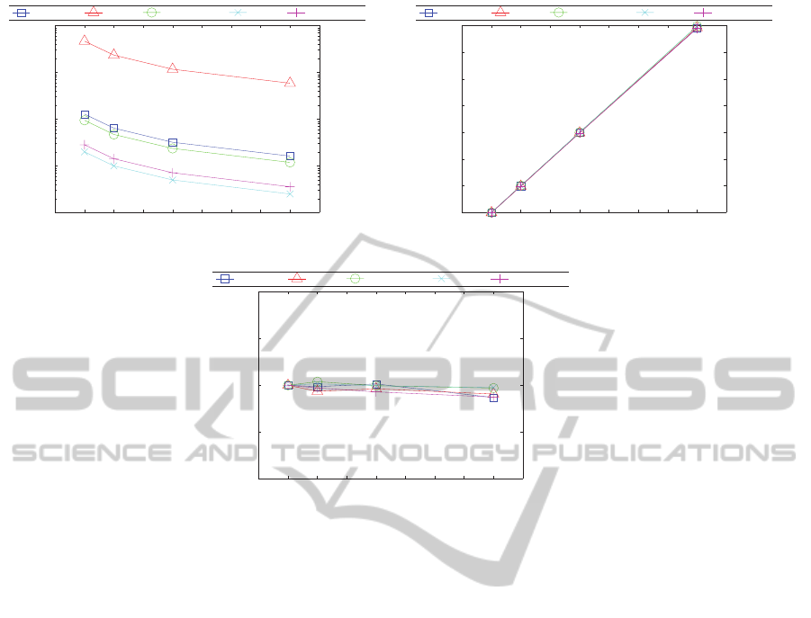
Finally, Figure 3 shows three graphs representing
the different measures related with the time perfor-
mance of the algorithm. Figure 3(a) plots the train-
ing time versus the number of nodes. Figure 3(b)
shows a graph of speedup factor against the number of
nodes. This form of display is often preferred to the
more obvious plot of training time versus the num-
ber of nodes, as it makes straightforward to see the
.
Table 3: Test accuracy (%).
Number of nodes
1 2 4 8
Madelon 71.38 71.27 71.05 70.82
MNIST 76.26 76.31 76.36 67.06
Mushrooms 93.25 92.04 91.81 91.78
Ozone 86.15 85.93 85.76 85.73
Spambase 88.78 88.72 88.76 88.81
impact on the training time of increasing the num-
ber of nodes. As can be deduced from Figure 3(c),
the efficiency of the proposed method is close to 1,
i.e. increasing the number of nodes by n divides the
training time by the same n. Notice the implications
of these results when dealing with high dimensional
datasets. The training time may be notably reduced
without compromising the classification accuracy. In
this manner,the proposed methodology allows to deal
with problems which were intractable with classical
approaches.
5 CONCLUSIONS
In this work, a new method for scaling up feature se-
lection was proposed. The idea was to vertically dis-
tribute the data and then performing a feature selec-
tion process which could be carried out at separate
nodes. Thus, the proposed methodology consists of
three different steps: discretization of the data, fea-
ture selection, and classification. All the stages are
executed in parallel and finally, the learned models
obtained from each node are combined in an incre-
mental manner. For this reason, the classical naive
Bayes classifier was modified so as to be able to make
it work incrementally.
The proposed methodology has been tested on five
datasets considered representative of problems from
medium to large size, and different numbers of nodes
to distribute the data were considered. As expected,
the larger the number of nodes, the shorter the time
required for the computation. However, in most of
the datasets, increasing the number of the nodes did
not lead to a significative degradation in classification
accuracy.
As future work, we plan to continue this research
using other feature selection algorithms and classi-
fiers, and trying another distributed approach where
all nodes share their results after each step (discretiza-
tion, feature selection and classification). In this
sense, the difficult of this future line of research lies
on the fact that for this approach, all the methods have
to be adapted to work in an incremental fashion.
LearningonVerticallyPartitionedDatabasedonChi-squareFeatureSelectionandNaiveBayesClassification
355
1 2 3 4 5 6 7 8
10
0
10
1
10
2
10
3
10
4
Number of nodes
Time (s)
Madelon MNIST Mushrooms Ozone Spambase
(a) Nodes vs time
1 2 3 4 5 6 7 8
1
2
3
4
5
6
7
8
Number of nodes
Speedup factor
Madelon MNIST Mushrooms Ozone Spambase
(b) Speed up
1 2 3 4 5 6 7 8
0.9
0.95
1
1.05
1.1
Number of nodes
Efficiency
Madelon MNIST Mushrooms Ozone Spambase
(c) Efficiency
Figure 3: Plots regarding time performance of the algorithm.
ACKNOWLEDGEMENTS
This research has been partially funded by the Sec-
retar´ıa de Estado de Investigaci´on of the Spanish
Government and FEDER funds of the European
Union through the research project TIN 2012-37954.
Ver´onica Bol´on-Canedo and Diego Peteiro-Barral ac-
knowledge the support of Xunta de Galicia under
Plan I2C Grant Program.
REFERENCES
Ananthanarayana, V., Subramanian, D., and Murty, M.
(2000). Scalable, distributed and dynamic mining
of association rules. High Performance Computing
HiPC 2000, pages 559–566.
Banerjee, M. and Chakravarty, S. (2011). Privacy preserv-
ing feature selection for distributed data using virtual
dimension. In Proceedings of the 20th ACM interna-
tional conference on Information and knowledge man-
agement, CIKM ’11, pages 2281–2284. ACM.
Bellman, R. (1966). Dynamic programming. Science,
153(3731):34–37.
Bol´on-Canedo, V., S´anchez-Maro˜no, N., and Alonso-
Betanzos, A. (2011). Feature selection and classifi-
cation in multiple class datasets: An application to
kdd cup 99 dataset. Expert Systems with Applications,
38(5):5947–5957.
Bramer, M. (2013). Dealing with large volumes of data. In
Principles of Data Mining, pages 189–208. Springer.
Chan, P., Stolfo, S., et al. (1993). Toward parallel and dis-
tributed learning by meta-learning. In AAAI workshop
in Knowledge Discovery in Databases, pages 227–
240.
Chawla, N. V., Hall, L. O., Bowyer, K. W., Moore Jr, T.,
and Kegelmeyer, W. P. (2002). Distributed pasting of
small votes. In Multiple Classifier Systems, pages 52–
61. Springer.
Chen, R., Sivakumar, K., and Kargupta, H. (2001). Dis-
tributed web mining using bayesian networks from
multiple data streams. In Data Mining, 2001. ICDM
2001, Proceedings IEEE International Conference on,
pages 75–82. IEEE.
Czarnowski, I. (2011). Distributed learning with data re-
duction. In Transactions on computational collective
intelligence IV, pages 3–121. Springer-Verlag.
de Haro Garc´ıa, A. (2011). Scaling data mining algorithms.
Application to instance and feature selection. PhD
thesis, Universidad de Granada.
Demˇsar, J. (2006). Statistical comparisons of classifiers
over multiple data sets. The Journal of Machine
Learning Research, 7:1–30.
Dunn, O. J. (1961). Multiple comparisons among
ICAART2014-InternationalConferenceonAgentsandArtificialIntelligence
356

means. Journal of the American Statistical Associa-
tion, 56(293):52–64.
Forman, G. (2003). An extensive empirical study of feature
selection metrics for text classification. The Journal
of Machine Learning Research, 3:1289–1305.
Frank, A. and Asuncion, A. (2010). UCI machine learning
repository.
Friedman, M. (1940). A comparison of alternative tests of
significance for the problem of m rankings. The An-
nals of Mathematical Statistics, 11(1):86–92.
Gangrade, A. and Patel, R. (2013). Privacy preserving
three-layer na¨ıve bayes classifier for vertically parti-
tioned databases. Journal of Information and Com-
puting Science, 8(2):119–129.
Guyon, I., Gunn, S., Nikravesh, M., and Zadeh, L. (2006).
Feature extraction: foundations and applications, vol-
ume 207. Springer.
Kantarcioglu, M. and Clifton, C. (2004). Privacy-
preserving distributed mining of association rules on
horizontally partitioned data. Knowledge and Data
Engineering, IEEE Transactions on, 16(9):1026–
1037.
Liu, H. and Setiono, R. (1995). Chi2: Feature selection
and discretization of numeric attributes. In Tools with
Artificial Intelligence, 1995. Proceedings., Seventh In-
ternational Conference on, pages 388–391. IEEE.
Liu, H. and Setiono, R. (1997). Feature selection via dis-
cretization. Knowledge and Data Engineering, IEEE
Transactions on, 9(4):642–645.
McConnell, S. and Skillicorn, D. (2004). Building predic-
tors from vertically distributed data. In Proceedings of
the 2004 conference of the Centre for Advanced Stud-
ies on Collaborative research, pages 150–162. IBM
Press.
Prodromidis, A., Chan, P., and Stolfo, S. (2000). Meta-
learning in distributed data mining systems: Issues
and approaches. Advances in distributed and paral-
lel knowledge discovery, 3.
Rish, I. (2001). An empirical study of the naive bayes clas-
sifier. In IJCAI 2001 workshop on empirical methods
in artificial intelligence, volume 3, pages 41–46.
Saari, P., Eerola, T., and Lartillot, O. (2011). Generaliz-
ability and simplicity as criteria in feature selection:
application to mood classification in music. Audio,
Speech, and Language Processing, IEEE Transactions
on, 19(6):1802–1812.
Saeys, Y., Inza, I., and Larra˜naga, P. (2007). A review of
feature selection techniques in bioinformatics. Bioin-
formatics, 23(19):2507–2517.
Skillicorn, D. and McConnell, S. (2008). Distributed pre-
diction from vertically partitioned data. Journal of
Parallel and Distributed computing, 68(1):16–36.
Tou, J. and Gonz´alez, R. (1977). Pattern recognition prin-
ciples. Addison-Wesley.
Tsoumakas, G. and Vlahavas, I. (2002). Distributed data
mining of large classifier ensembles. In Proceedings
Companion Volume of the Second Hellenic Confer-
ence on Artificial Intelligence, pages 249–256.
Tsoumakas, G. and Vlahavas, I. (2009). Distributed data
mining. Database Technologies: Concepts, Method-
ologies, Tools, and Applications, 1:157.
Vaidya, J. and Clifton, C. (2004). Privacy preserving na¨ıve
bayes classifier for vertically partitioned data. In 2004
SIAM International Conference on Data Mining, Lake
Buena Vista, Florida, pages 522–526.
Vaidya, J. and Clifton, C. (2005). Privacy-preserving deci-
sion trees over vertically partitioned data. In Data and
Applications Security XIX, pages 139–152. Springer.
Ventura, D. and Martinez, T. (1995). An empirical com-
parison of discretization methods. In Proceedings of
the Tenth International Symposium on Computer and
Information Sciences, pages 443–450.
Wang, J., Luo, Y., Zhao, Y., and Le, J. (2009). A survey on
privacy preserving data mining. In Database Technol-
ogy and Applications, 2009 First International Work-
shop on, pages 111–114. IEEE.
Wirth, R., Borth, M., and Hipp, J. (2001). When distribu-
tion is part of the semantics: A new problem class for
distributed knowledge discovery. In Proceedings of
the PKDD 2001 workshop on ubiquitous data mining
for mobile and distributed environments, pages 56–64.
Citeseer.
Wolpert, D. H. (1992). Stacked generalization. Neural net-
works, 5(2):241–259.
Yao, A. C. (1982). Protocols for secure computations. In
Proceedings of the 23rd Annual Symposium on Foun-
dations of Computer Science, pages 160–164.
Ye, M., Hu, X., and Wu, C. (2010). Privacy preserving
attribute reduction for vertically partitioned data. In
Artificial Intelligence and Computational Intelligence
(AICI), 2010 International Conference on, volume 1,
pages 320–324. IEEE.
Zhao, Z. and Liu, H. (2011). Spectral Feature Selection for
Data Mining. Chapman & Hall/Crc Data Mining and
Knowledge Discovery. Taylor & Francis Group.
LearningonVerticallyPartitionedDatabasedonChi-squareFeatureSelectionandNaiveBayesClassification
357
